Comparing ORBSLAM3 results of multiple runs graphically
Tables of mean, RMSE, median and standard deviations might not be the most useful analysis tool when the error distribution is not known. Graphs of the distribution shapes might be more informative.
In this experiment, I will inspect the result from the previous post in a graphical way. That the mean and median ATEs are not roughly equal for each run is an indication that we are dealing with non-Gaussian error distributions. This, in turn, means that the mean and standard deviation are not sufficient descriptive statistics to summarise these error distributions.
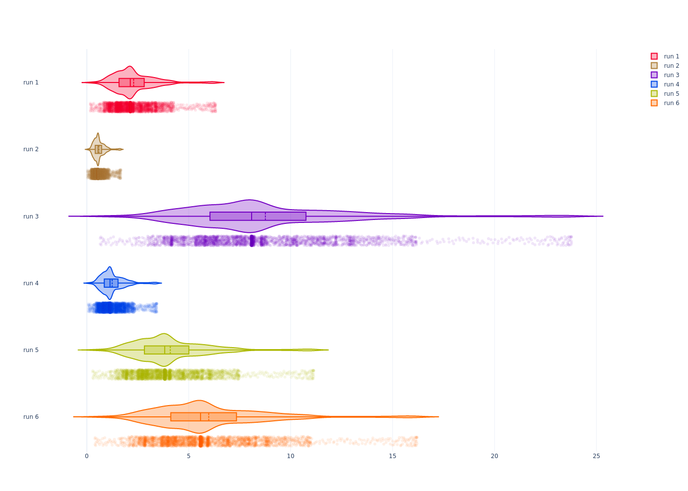
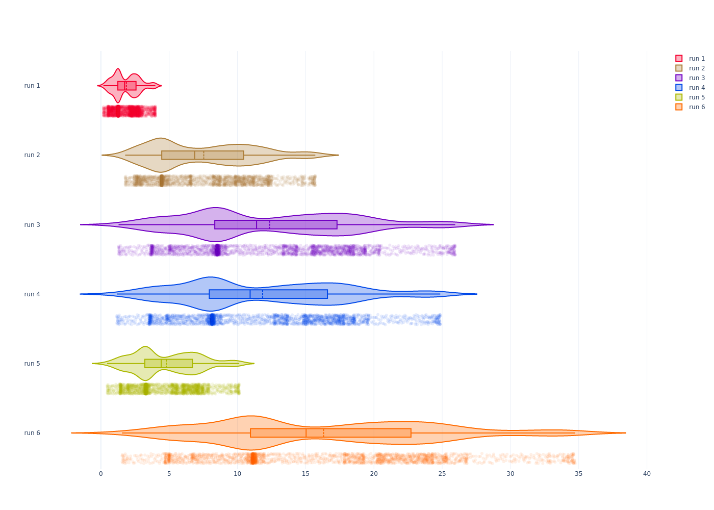
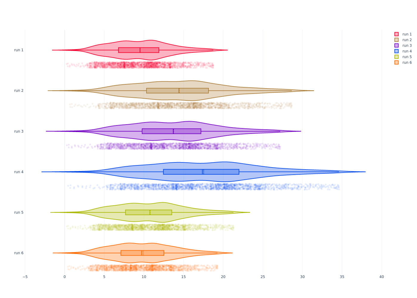
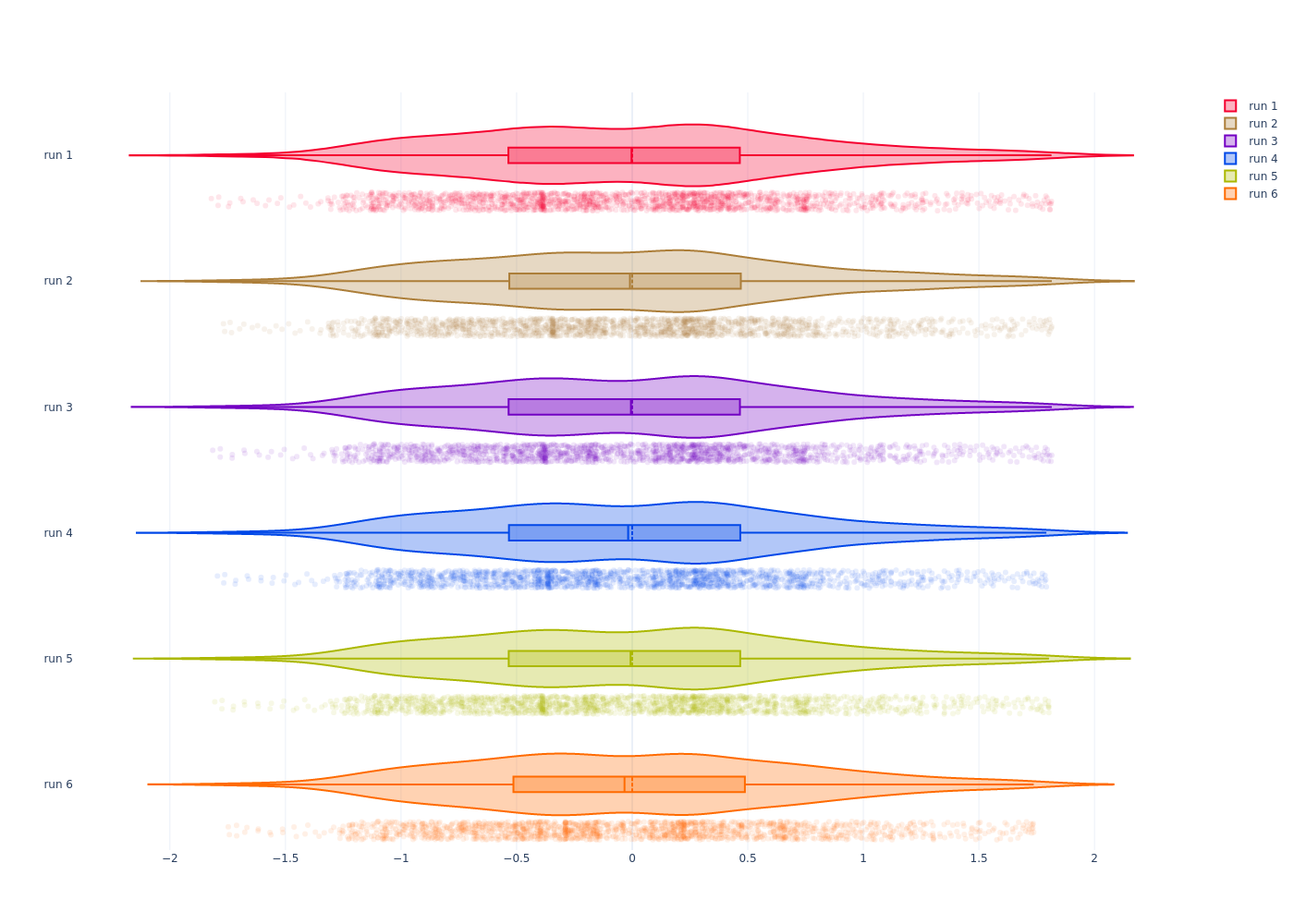
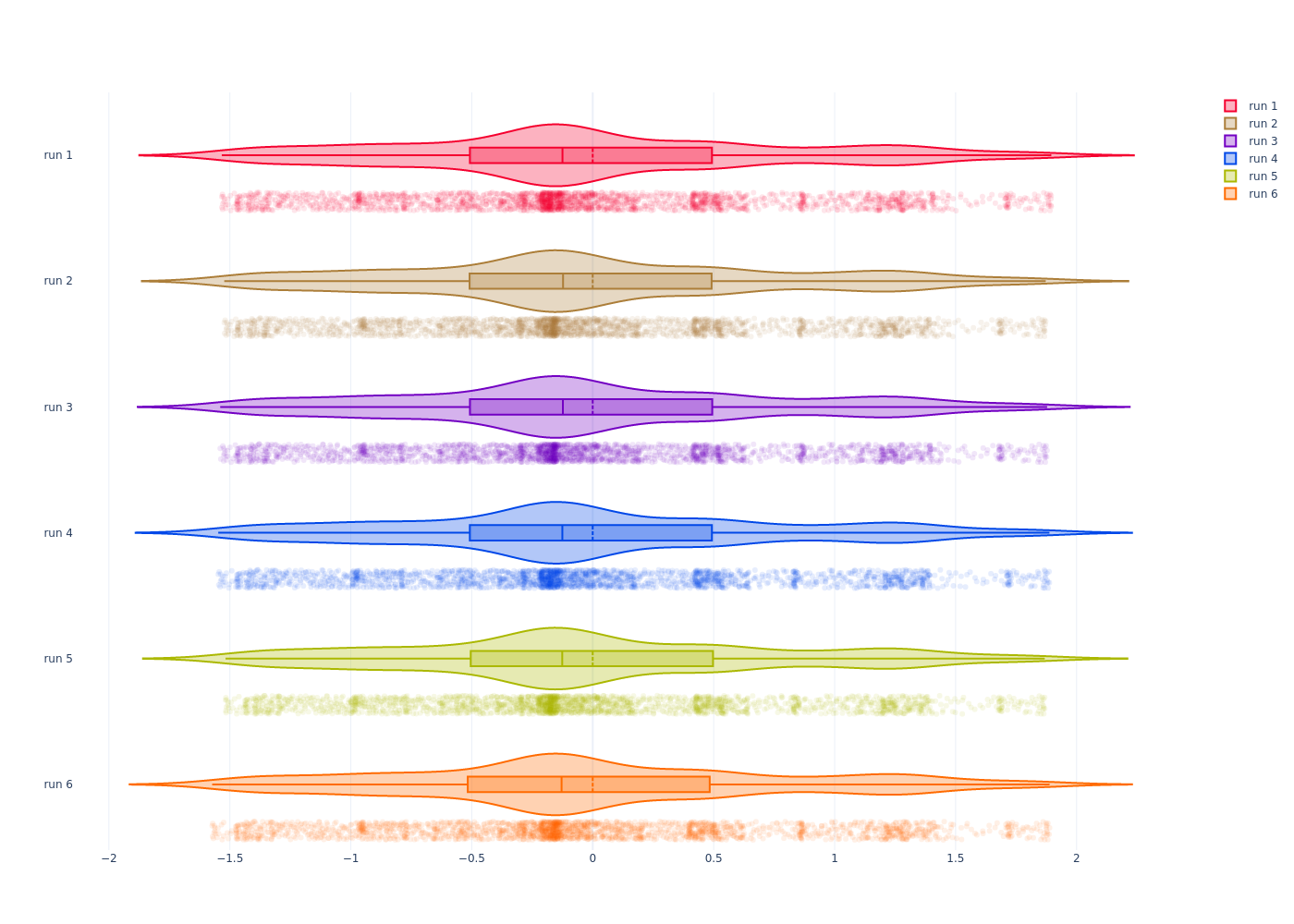
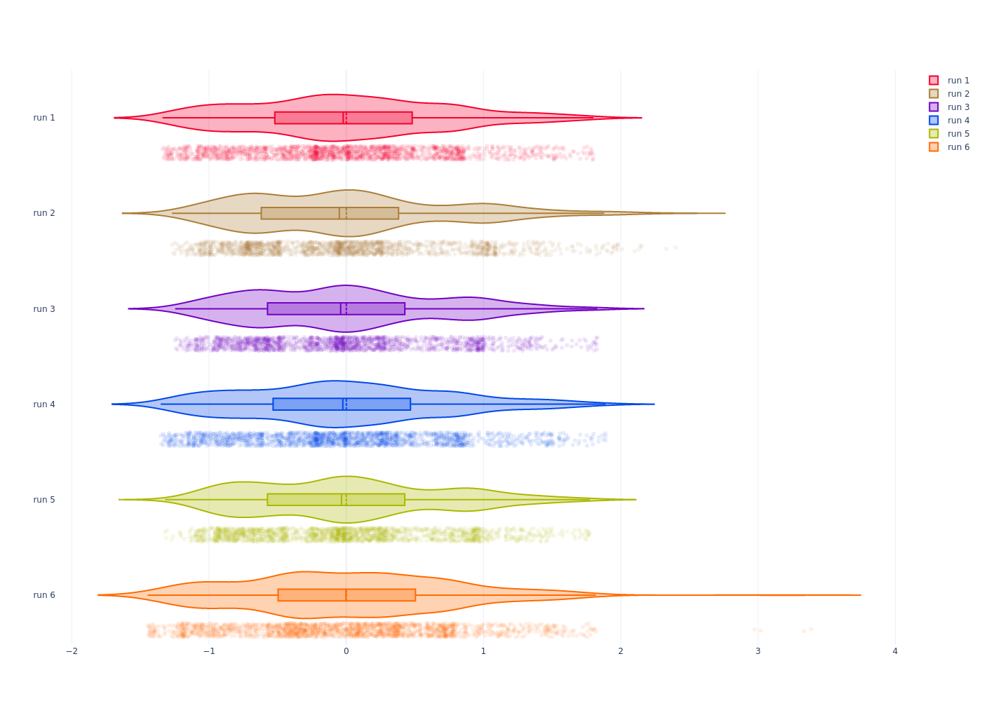
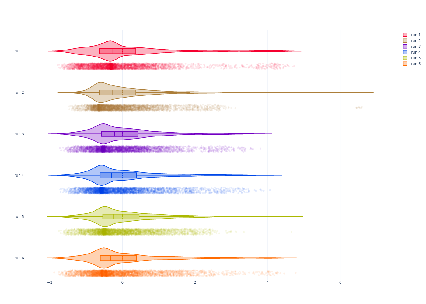
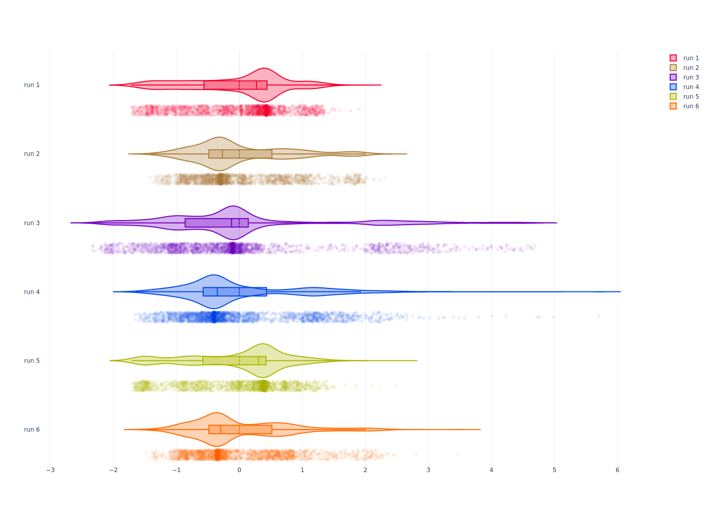
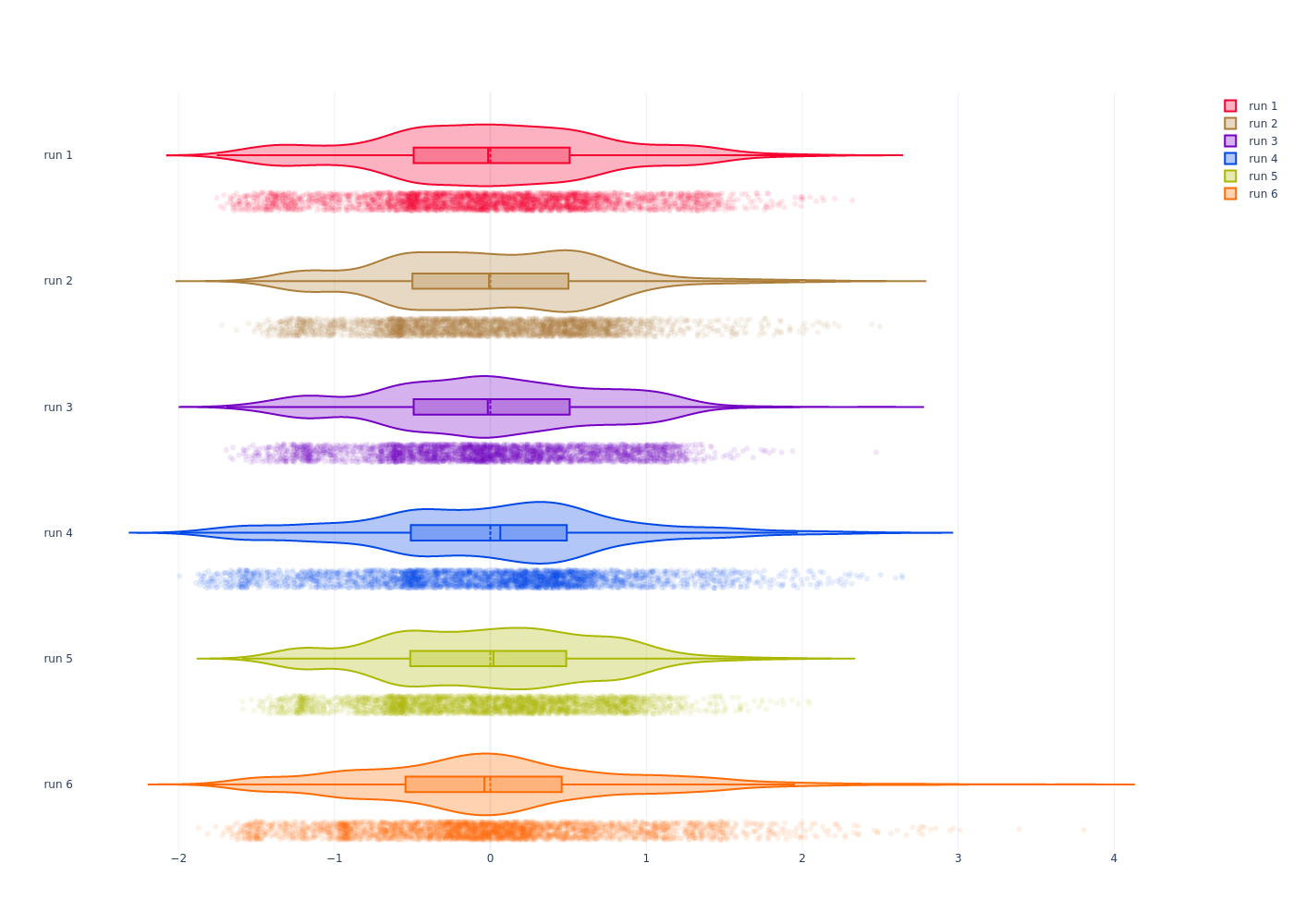
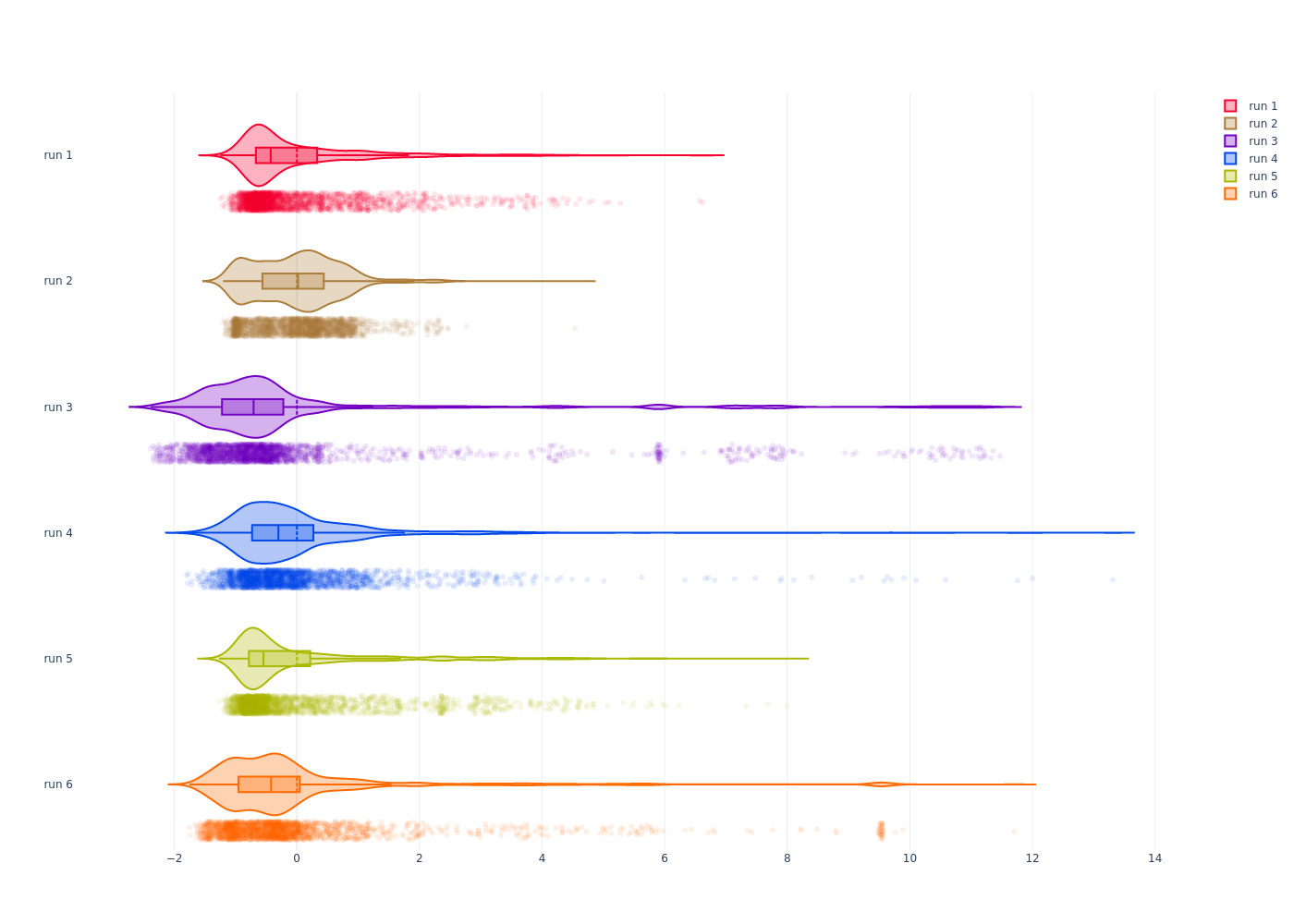
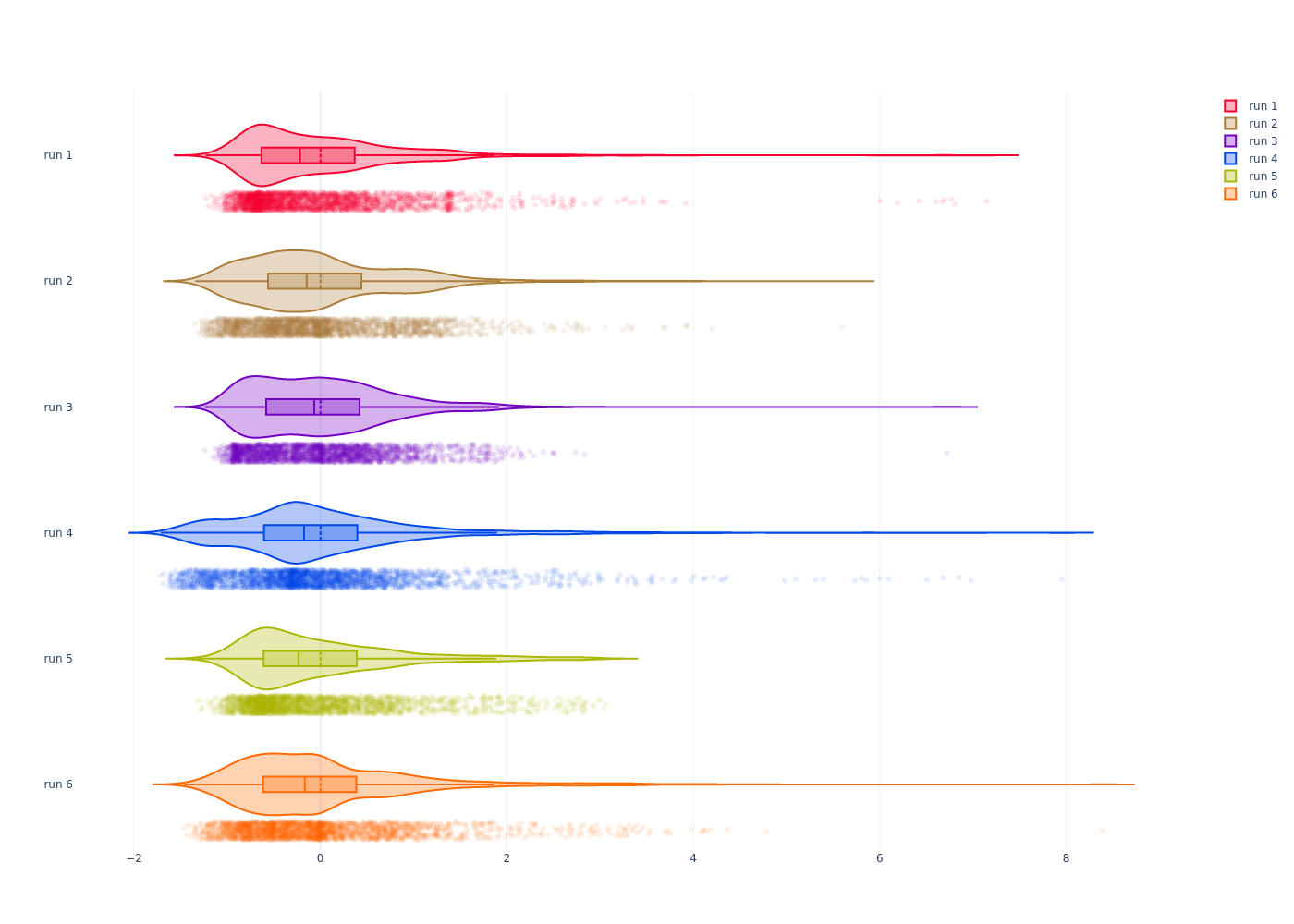
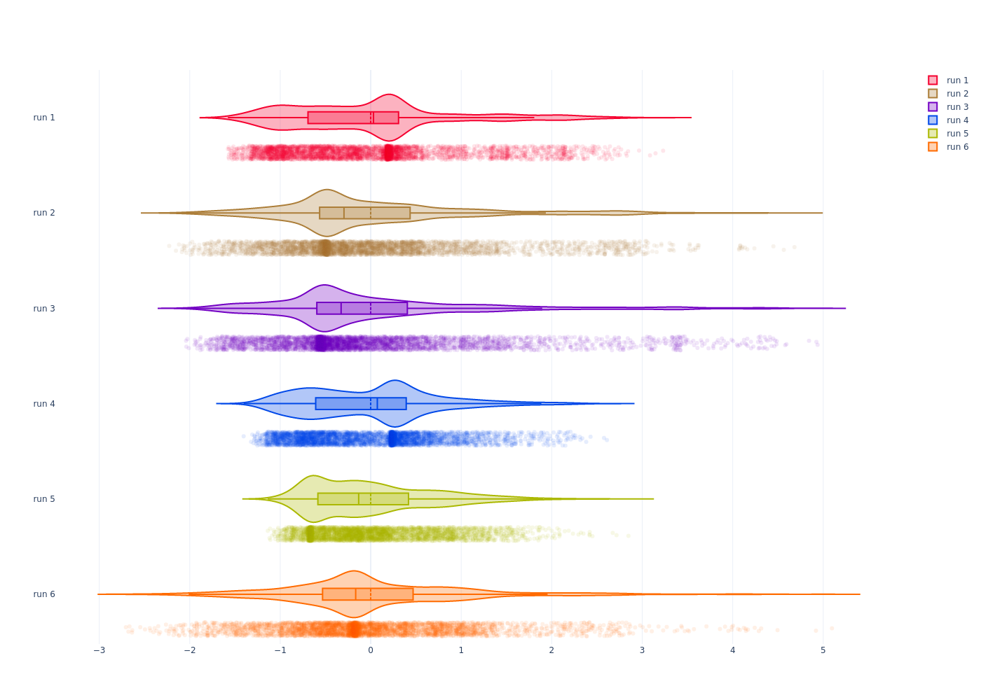
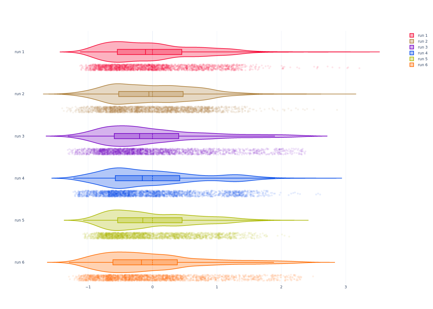
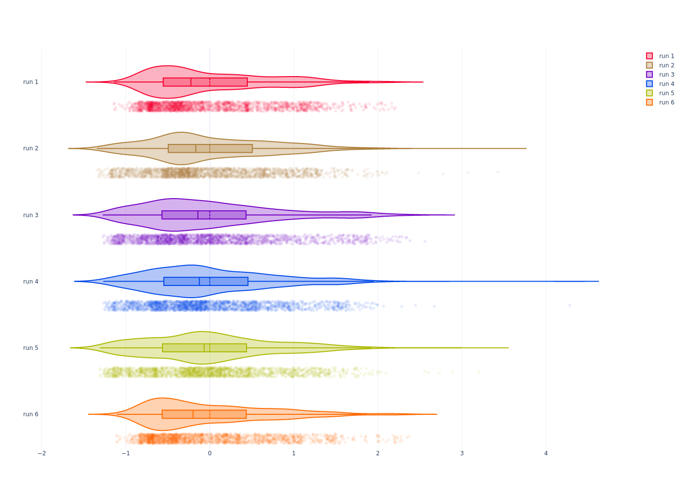
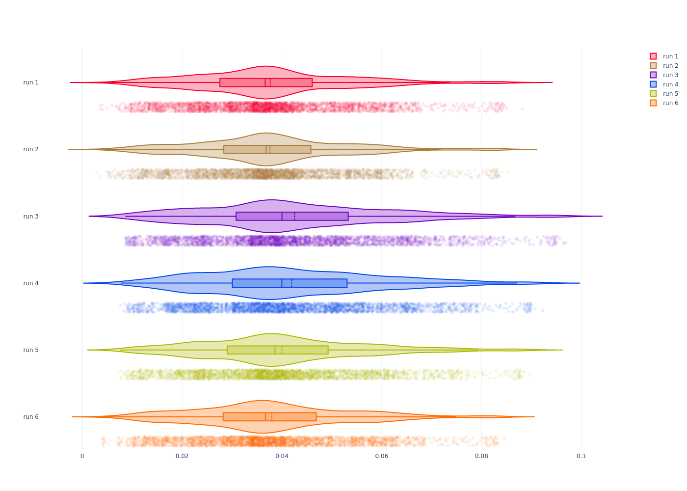
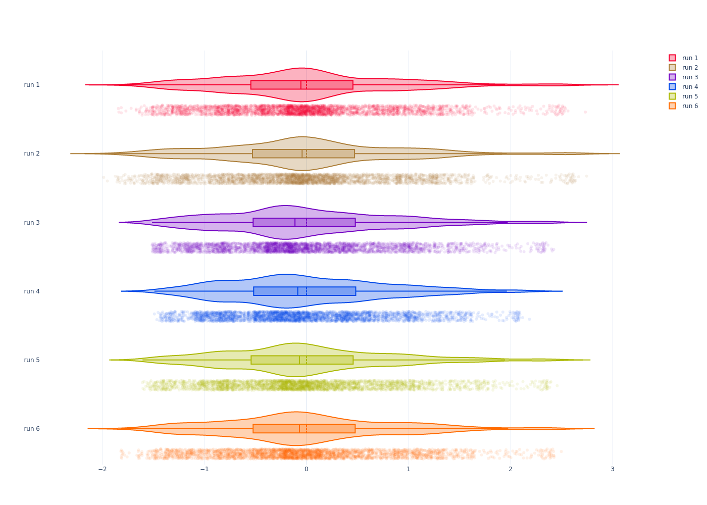
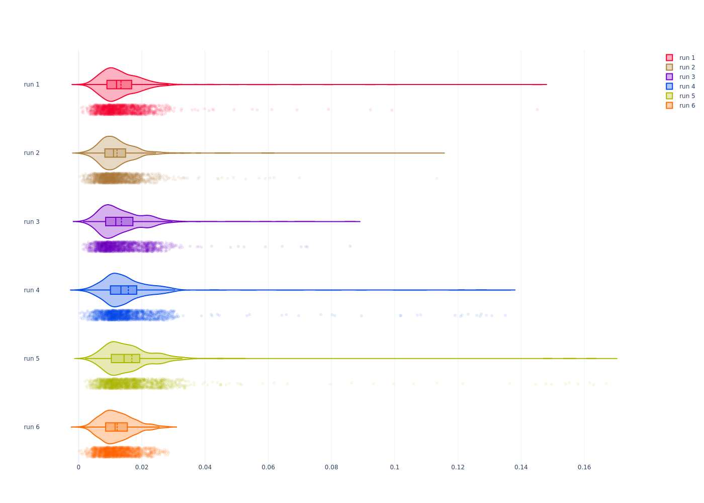
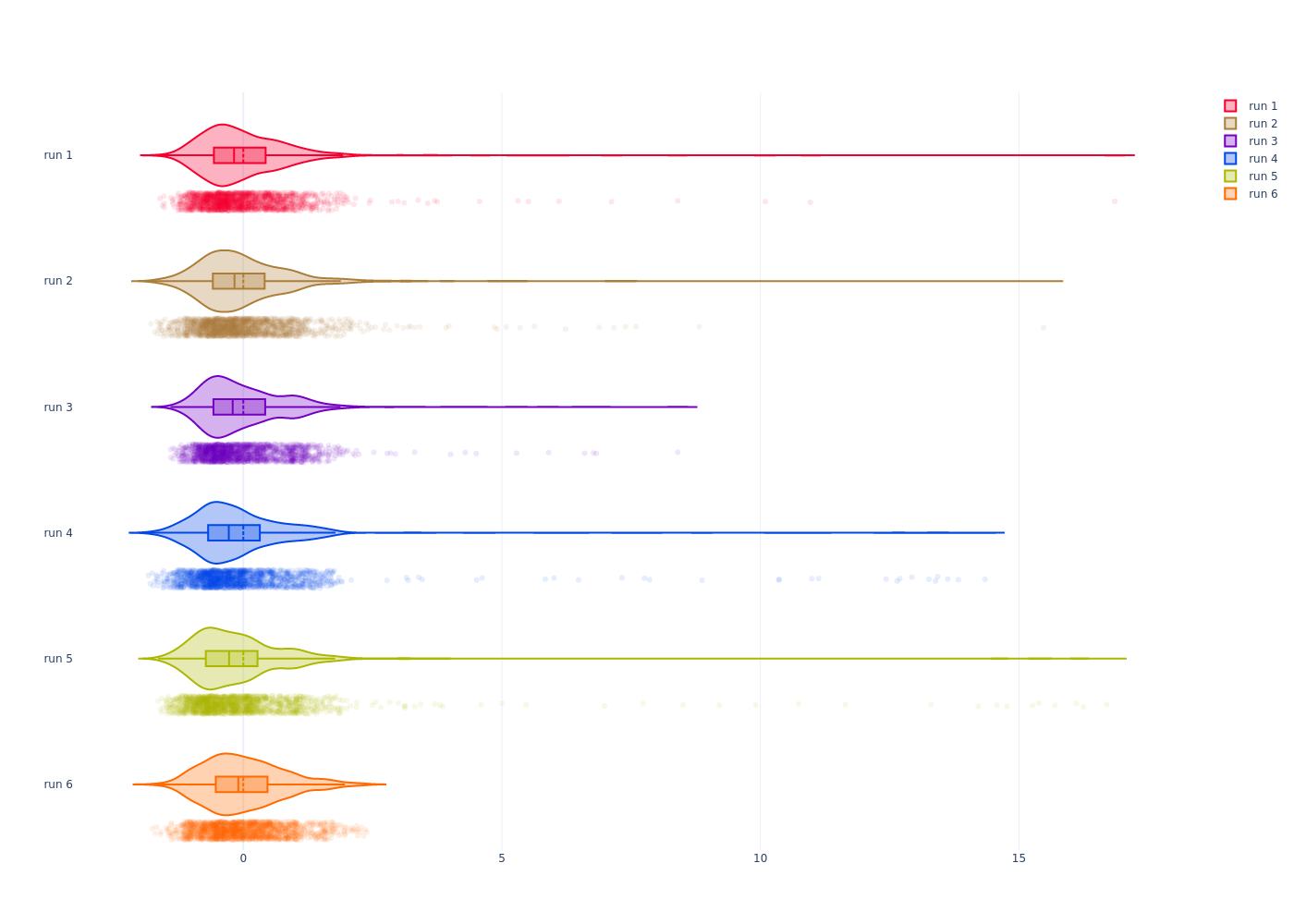
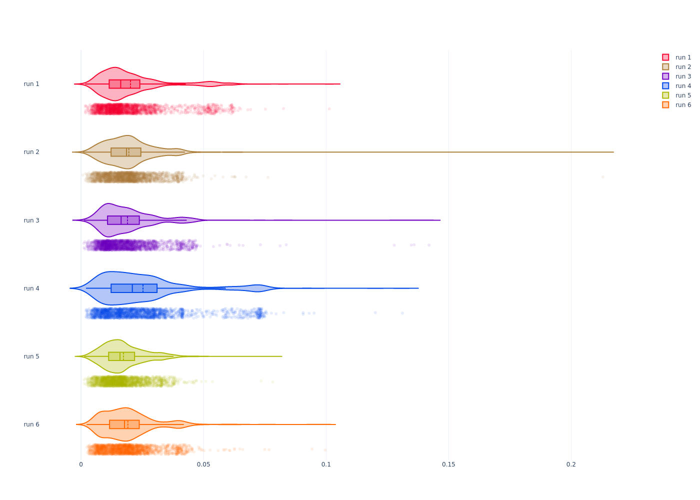
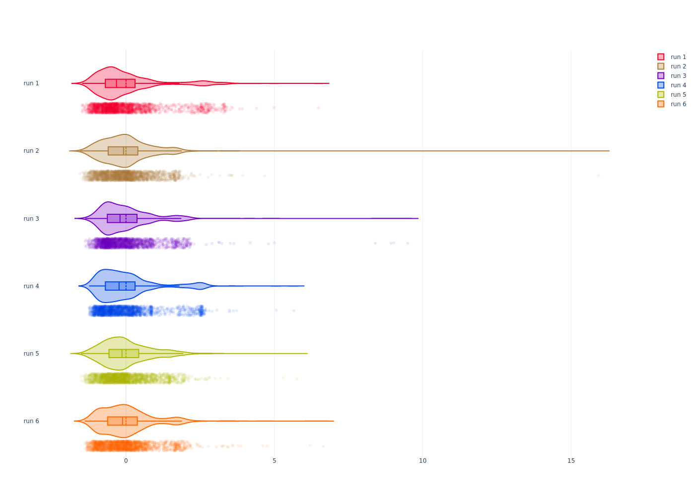
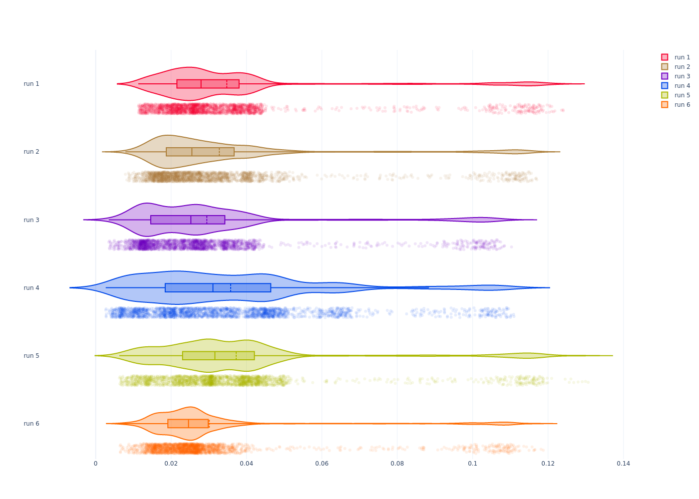
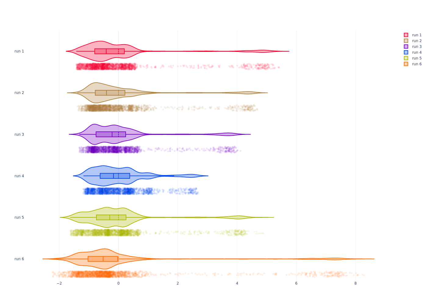
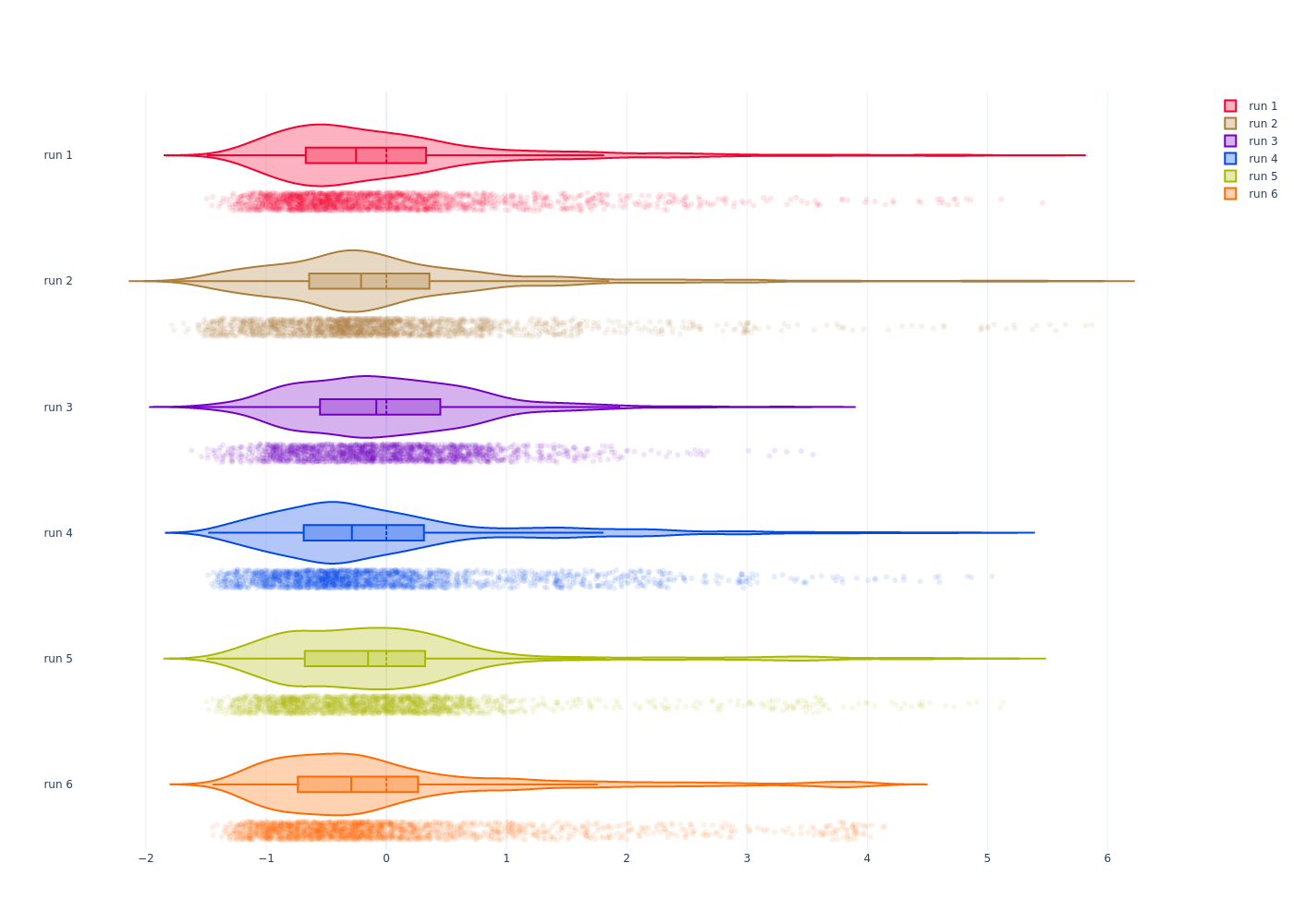
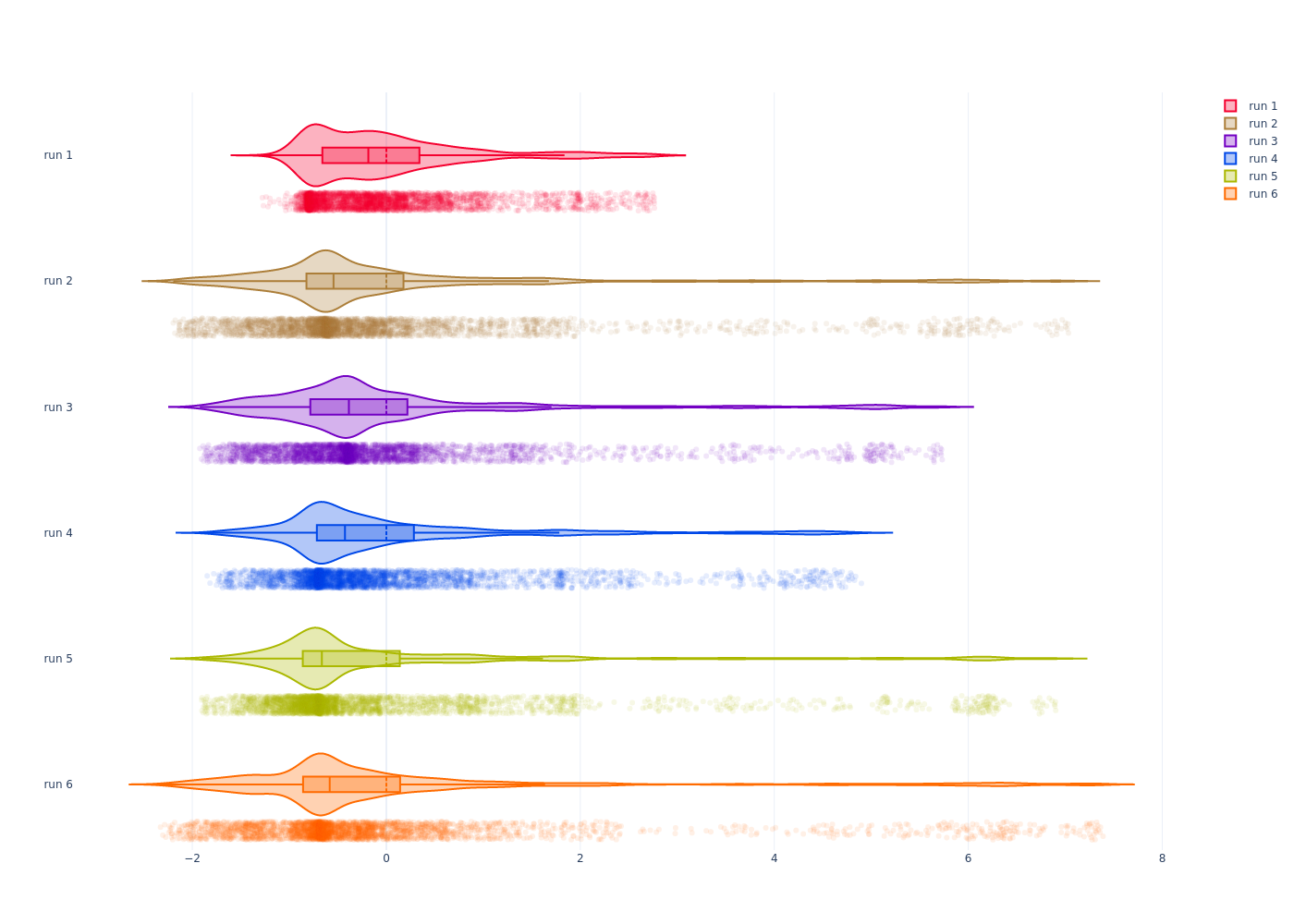
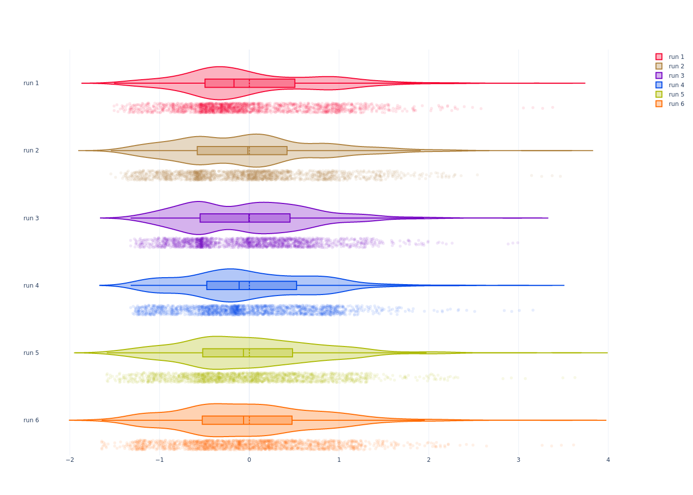
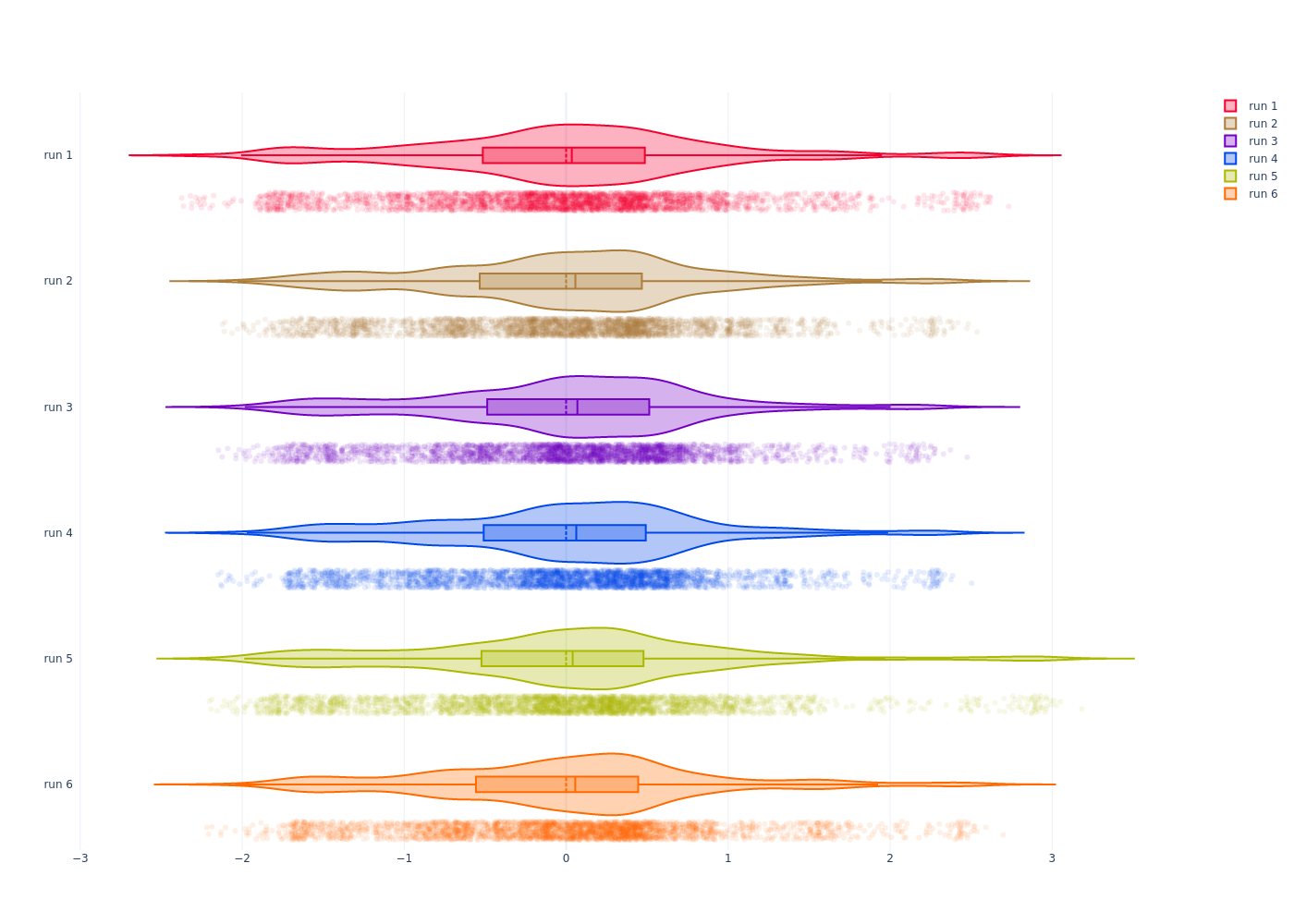
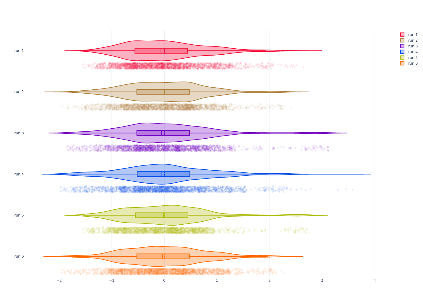
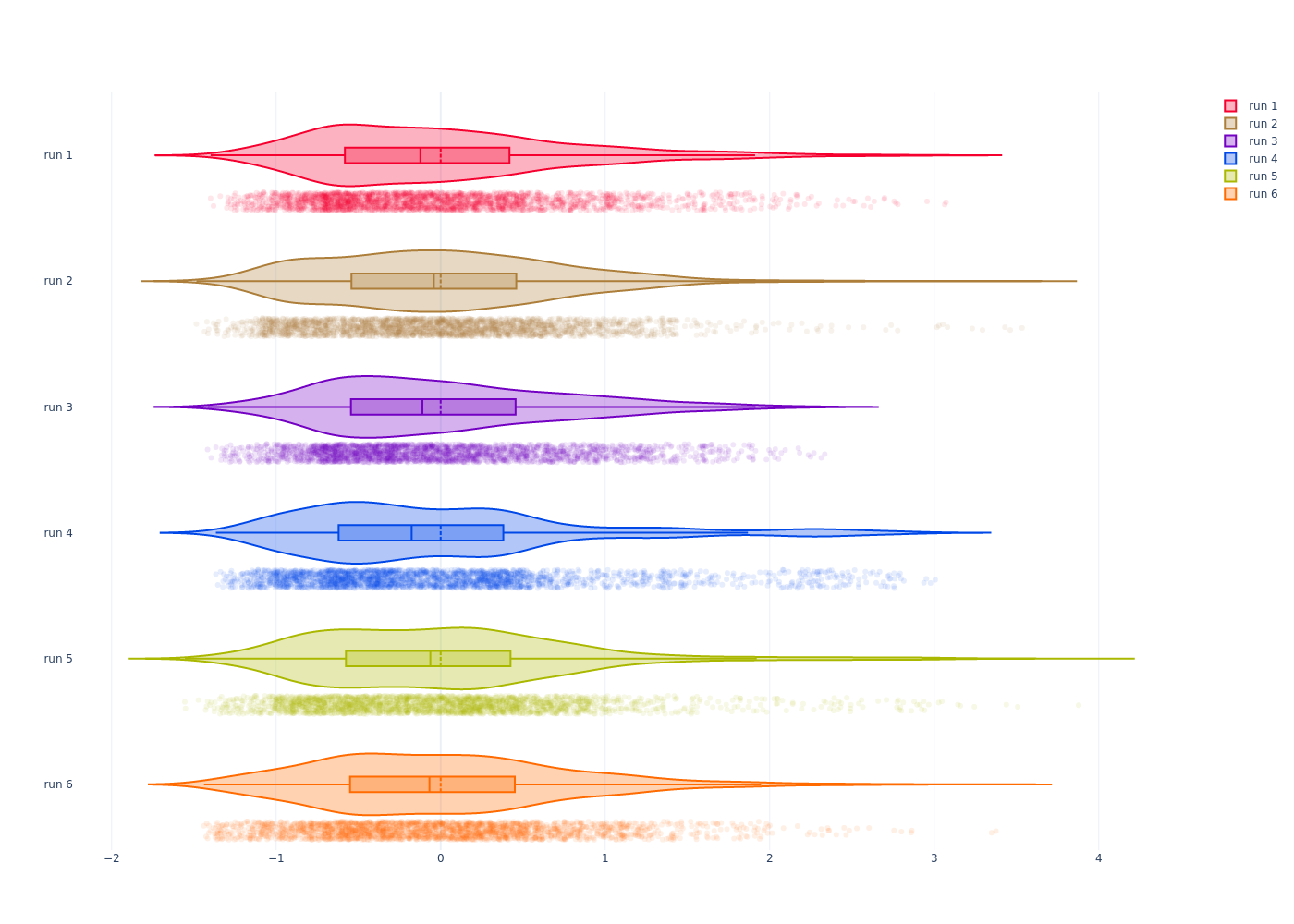
In the below figures, each first subfigure presents violin plots (with inside the violin bodies a box plot) and scatter plots of the ATE distributions. Runs from the same sensor mode and dataset are grouped together, as error distributions between runs of different sensor modes and datasets are expected to be different (as each dataset contains a different number of challenging scenes for each sensor mode). The violin plots and scatter plots show that the error distributions are indeed non-Gaussian.
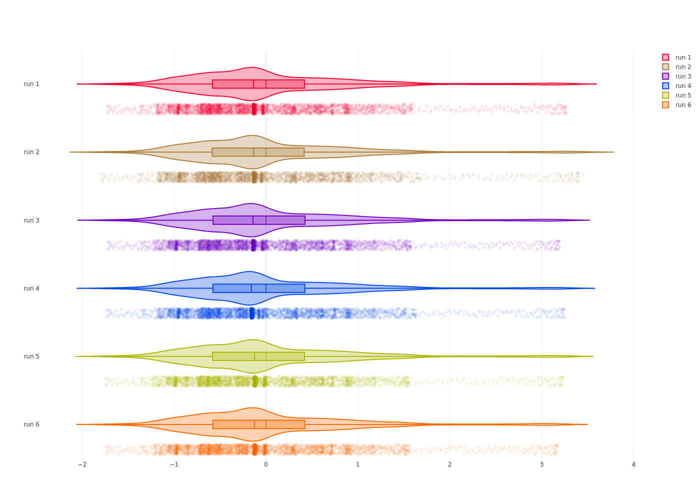
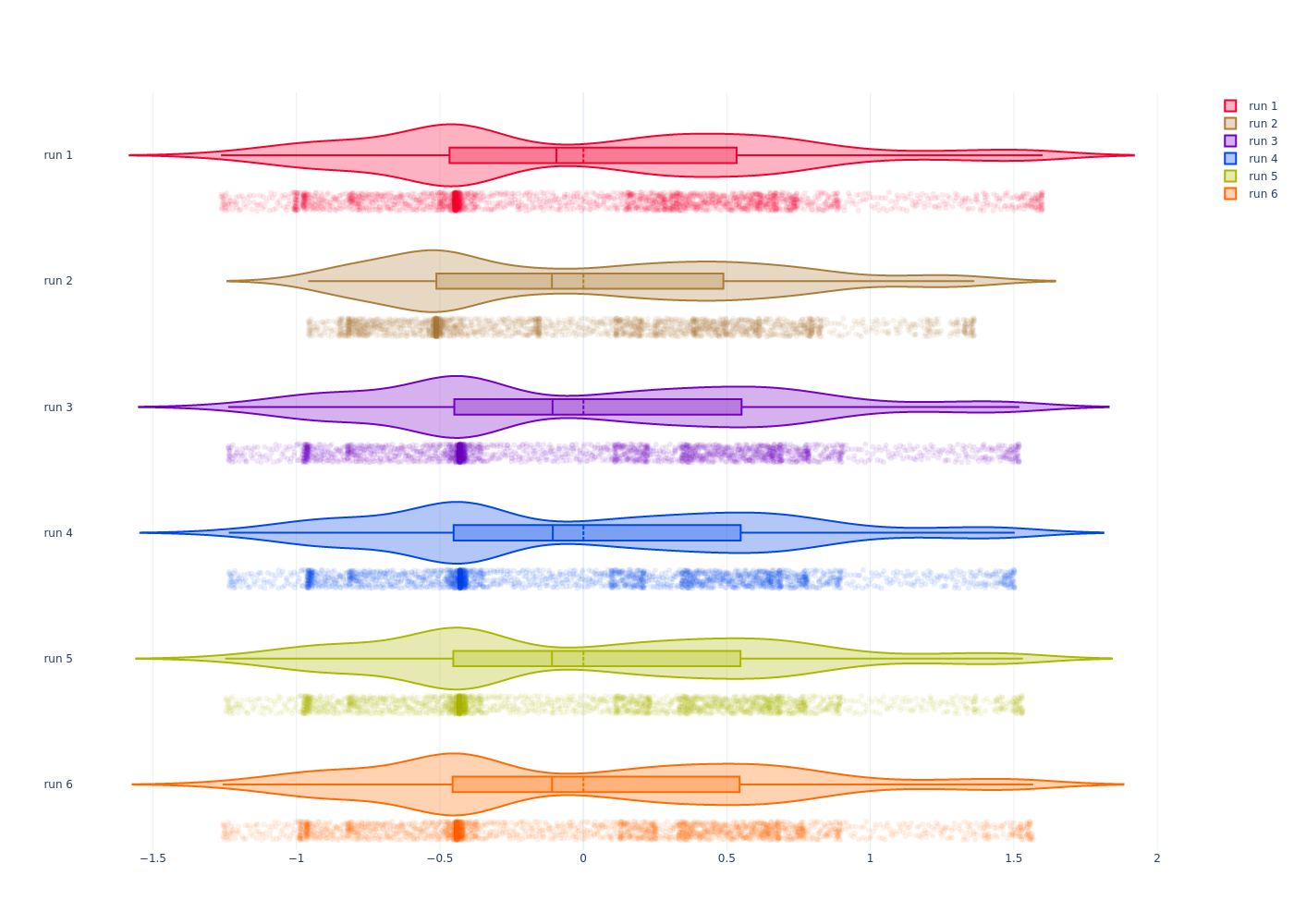
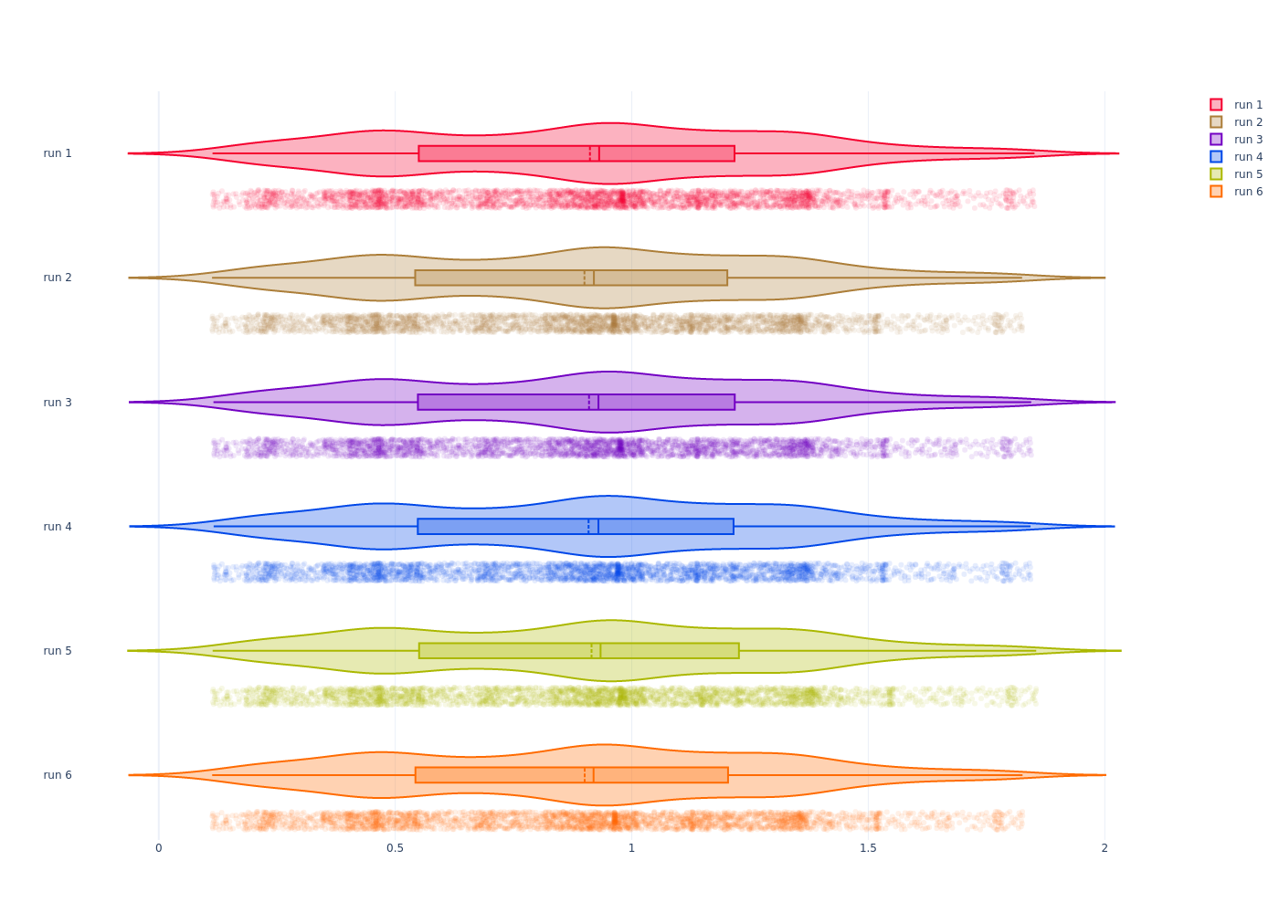
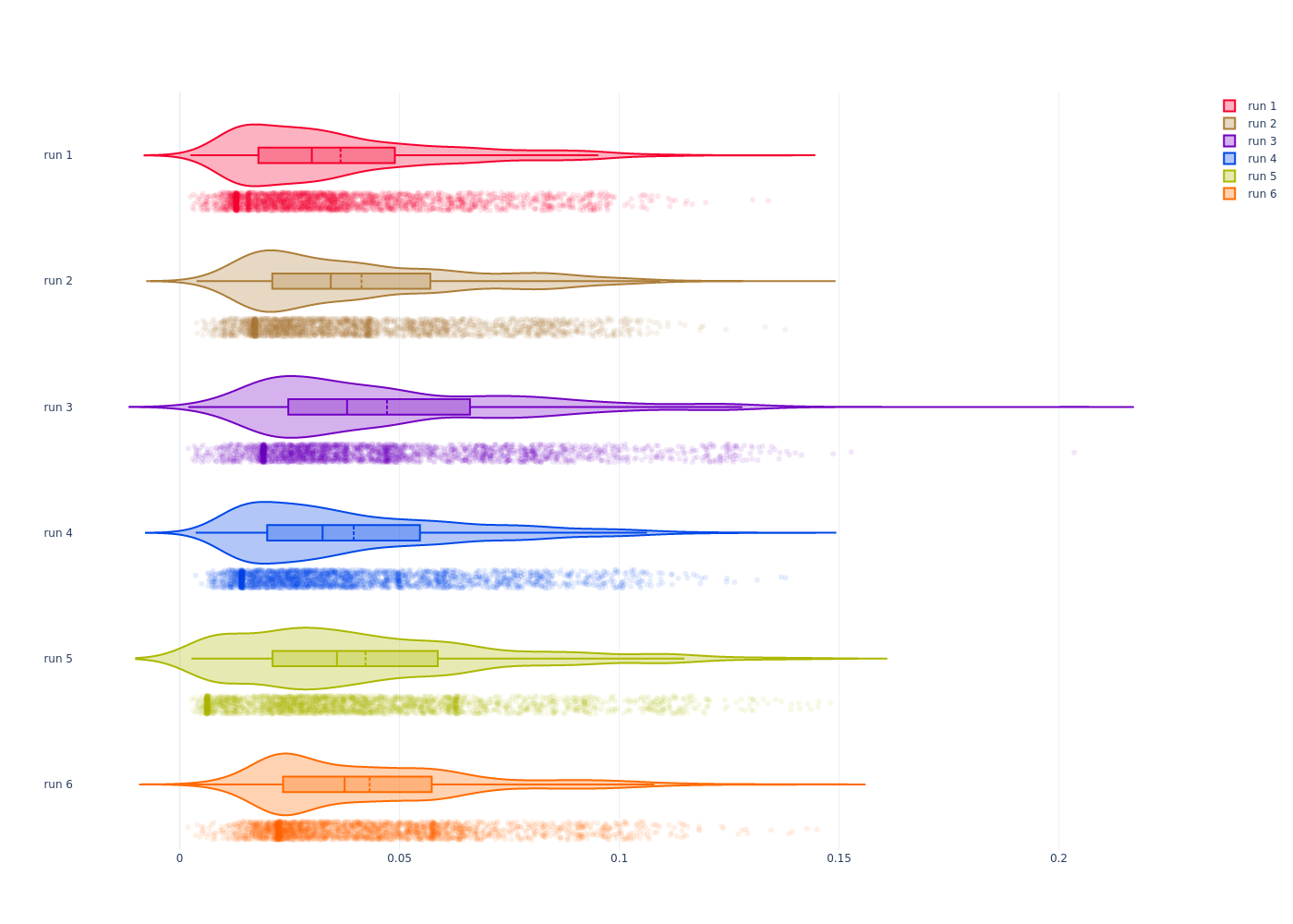
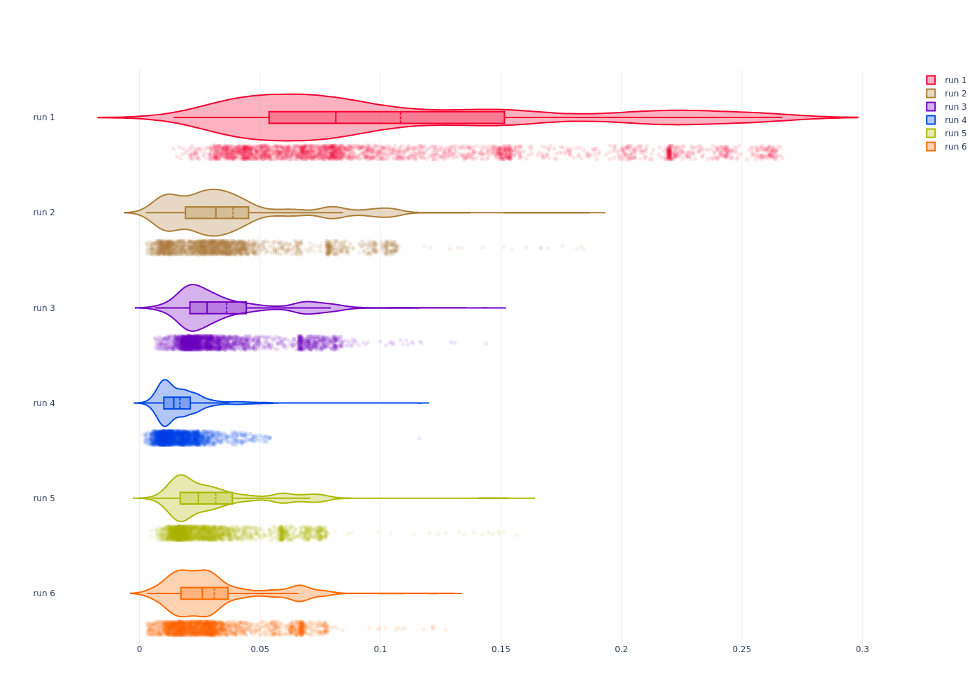
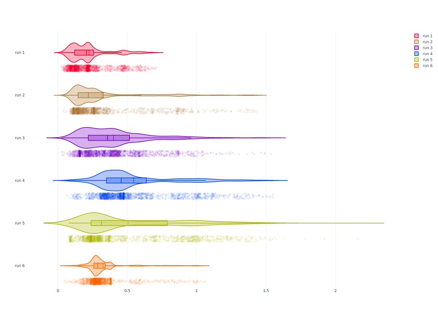
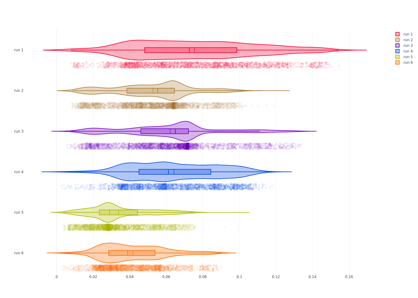
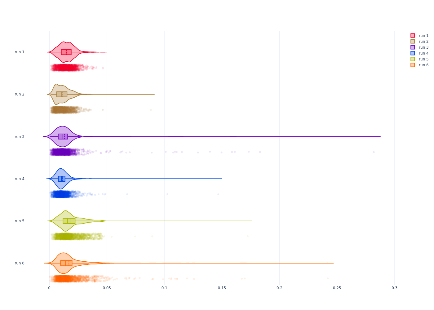
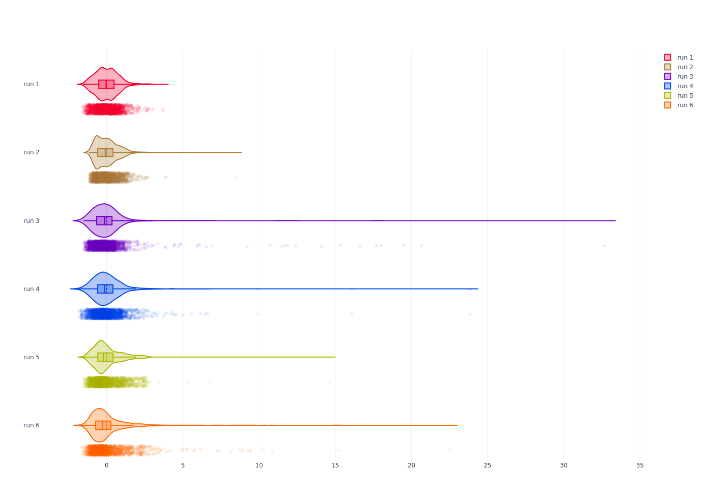
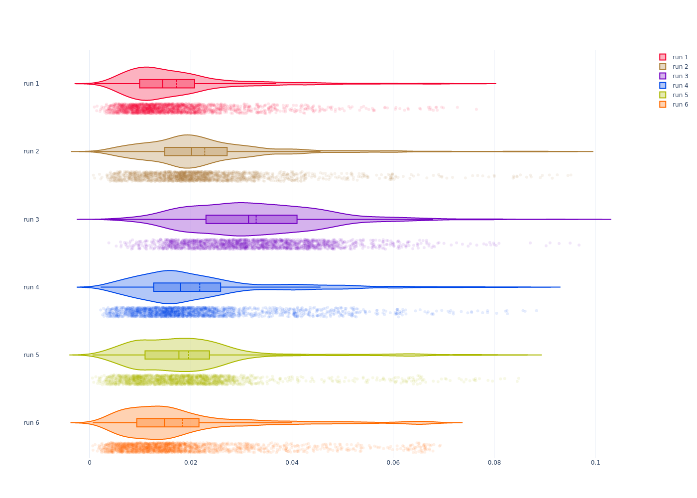
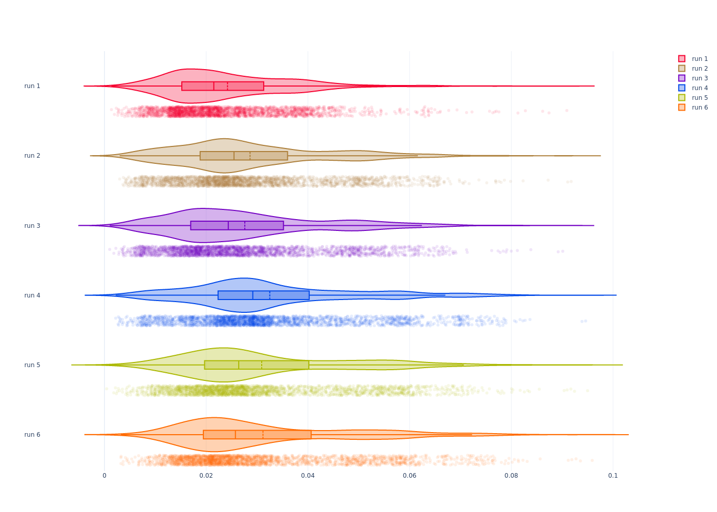
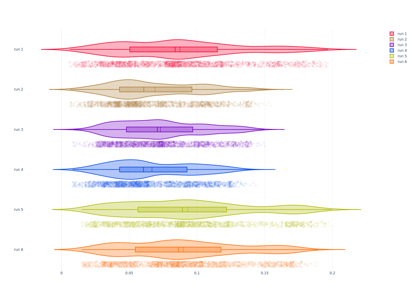
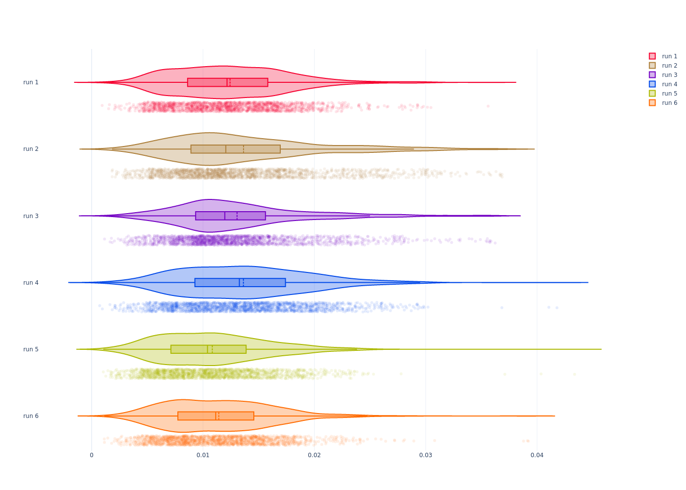
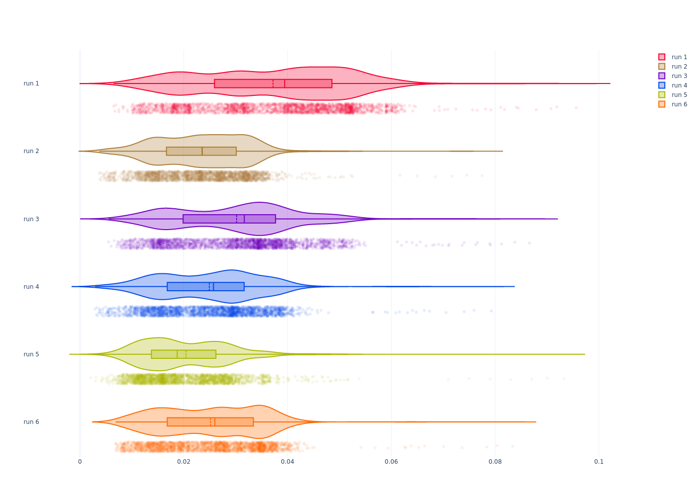
In each figure, a second subfigure is included. In these graphs, the ATEs are normalized such that the interquartile range \(r = Q_3 - Q_1\) equals 1, and the mean \(\mu\) is set to 0. That is, for each error \(e\), the normalized error \(\bar{e} = \frac{e - \mu}{r}\). By normalizing, it is easier to compare visually if the errors originate from similar underlying distributions. If that would be the case, the shape of all violins in each second subfigure should look very much alike. In those cases, the difference between ATEs of different runs can be attributed to small errors in initialization due to the ORBSLAM framework’s multithreadedness, and failing to recognise the same (metric) scale of the physical environment. The least variation in violin shape is expected for the monocular case, as this sensor mode has no method of knowing the true metric scale. In the stereo case, metric information can be retrieved through parallax, which is a more stable method than the inertial scale retrieval mode used in the final two options. With those two sensor modes, I expect a similar amount of variation in violin shape.
To truly make hard claims about this vague term of „violin shape”, I need some way to compare their shapes in a quantitive way (as opposed to this qualitative analysis). Right now, I’m using the Mann-Whitney U test, but I am not sure if that is the right test I am looking for.
Monocular
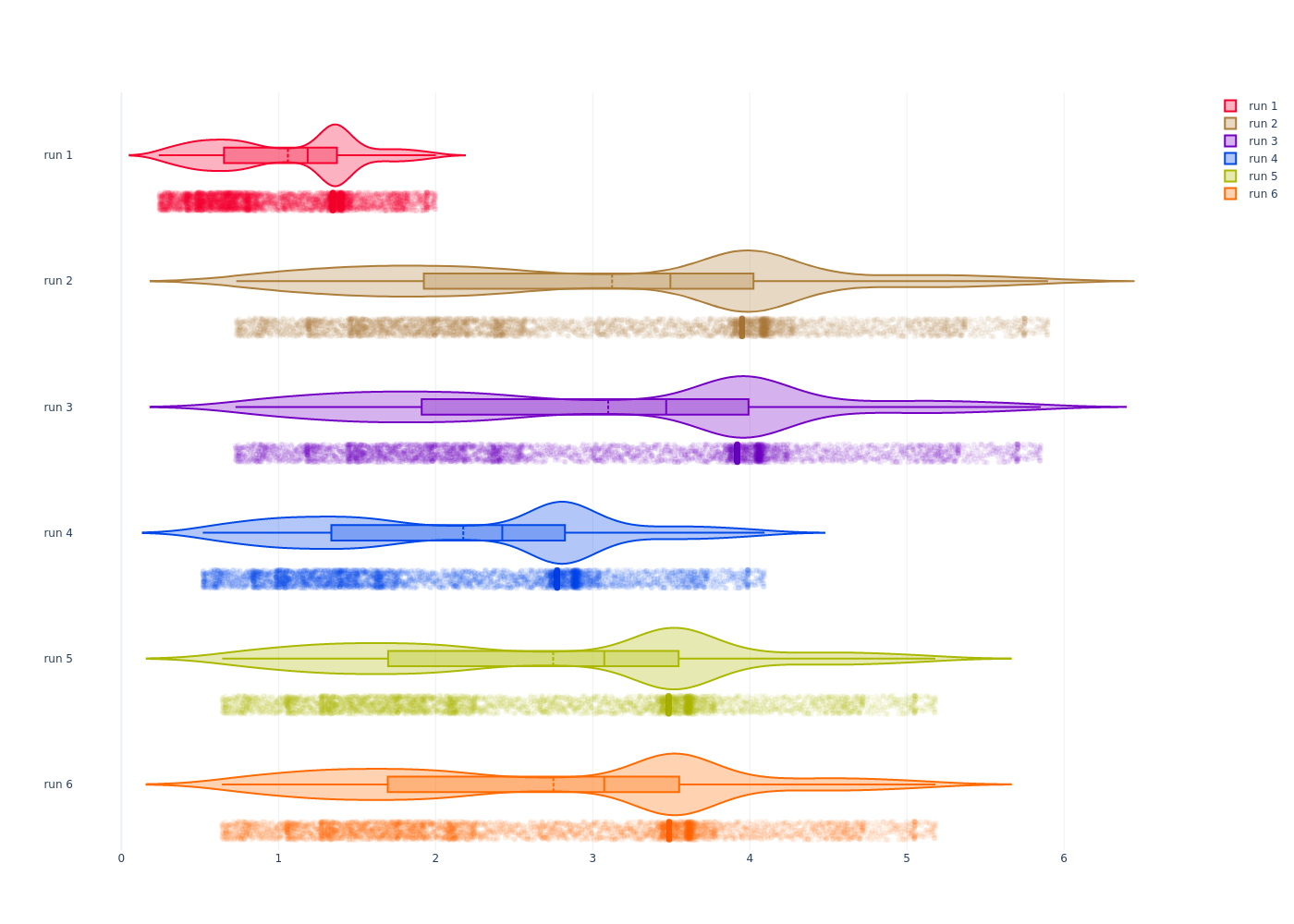
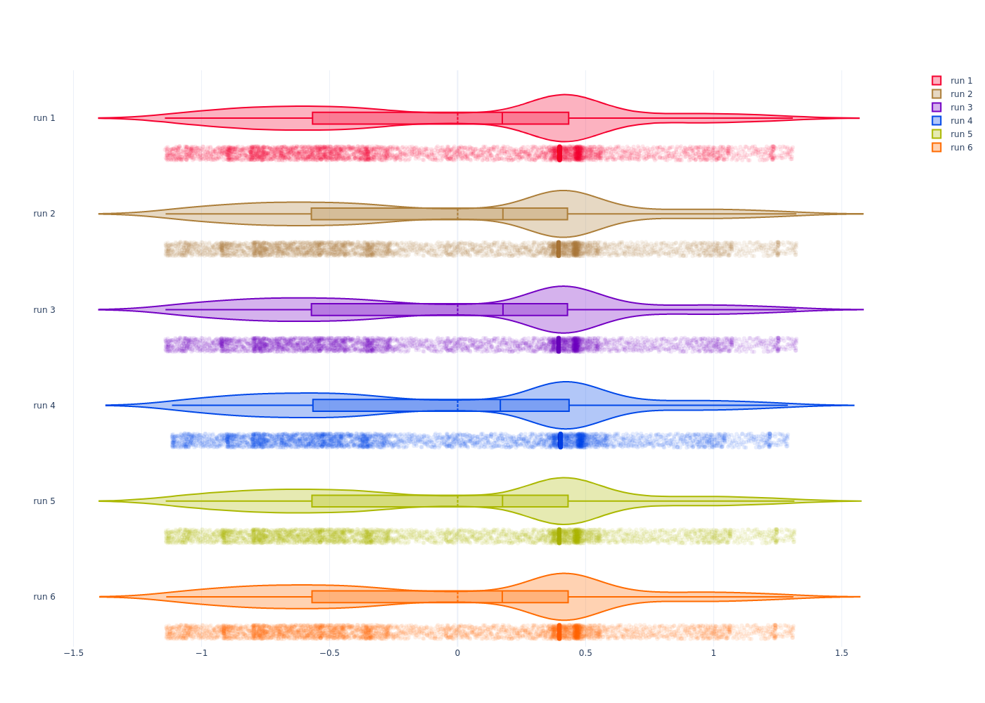
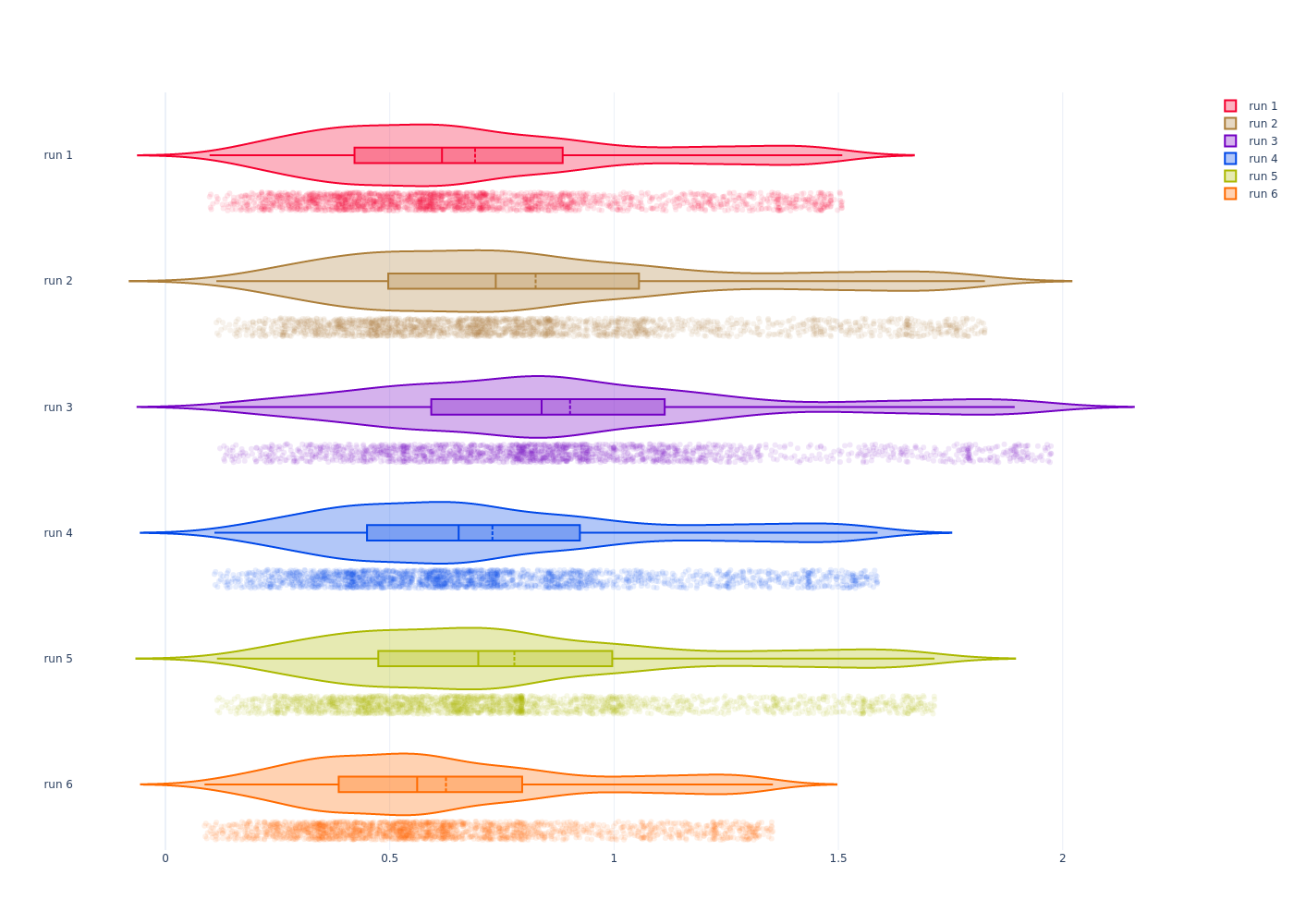
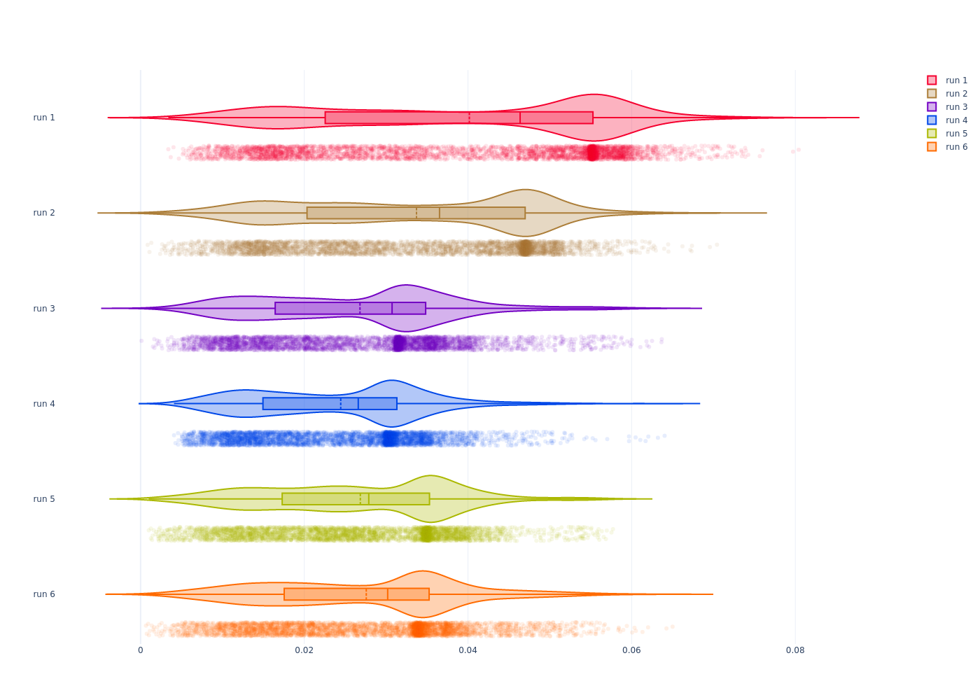
Violin plot, showing the error distributions for monocular runs 1 through 6 for the EuRoC MH01 dataset. Left: not normalized. Right: each run is normalized by its interquartile range, and its mean is set to 0.
Mann-Whitney U test
| run 1 | run 2 | run 3 | run 4 | run 5 | run 6 | |
|---|---|---|---|---|---|---|
| run 1 | 0.999996 | 0 | 0 | 0 | 0 | 0 |
| run 2 | 0 | 0.999996 | 0.00473279 | 8.74955e-210 | 4.38792e-51 | 4.76644e-51 |
| run 3 | 0 | 0.00473279 | 0.999996 | 9.12142e-204 | 1.38488e-47 | 1.34058e-47 |
| run 4 | 0 | 8.74955e-210 | 9.12142e-204 | 0.999996 | 8.72346e-111 | 7.88491e-111 |
| run 5 | 0 | 4.38792e-51 | 1.38488e-47 | 8.72346e-111 | 0.999996 | 0.123 |
| run 6 | 0 | 4.76644e-51 | 1.34058e-47 | 7.88491e-111 | 0.123 | 0.999996 |
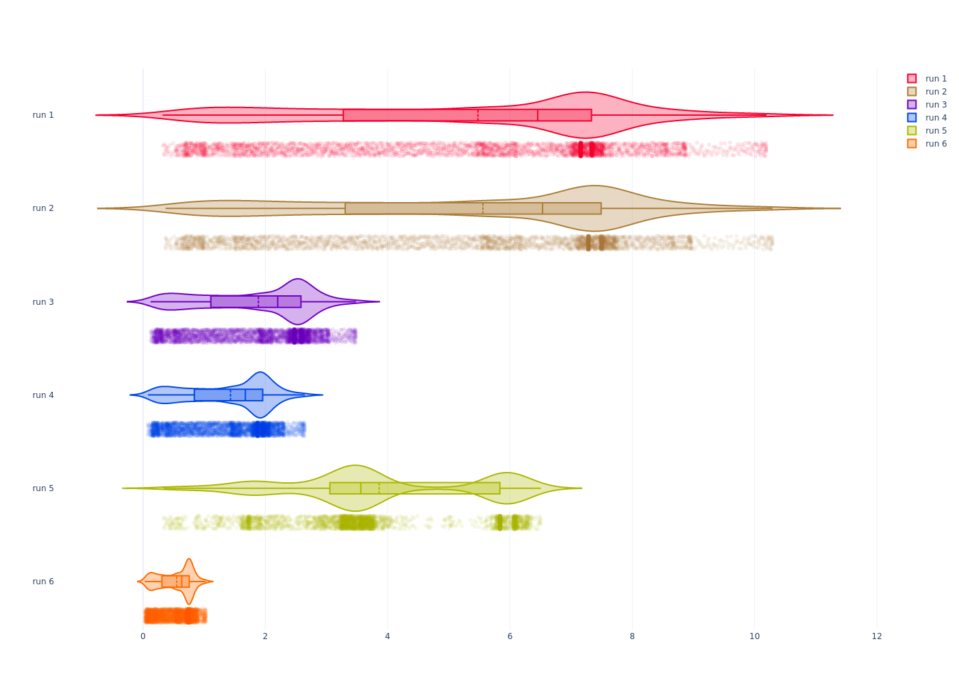
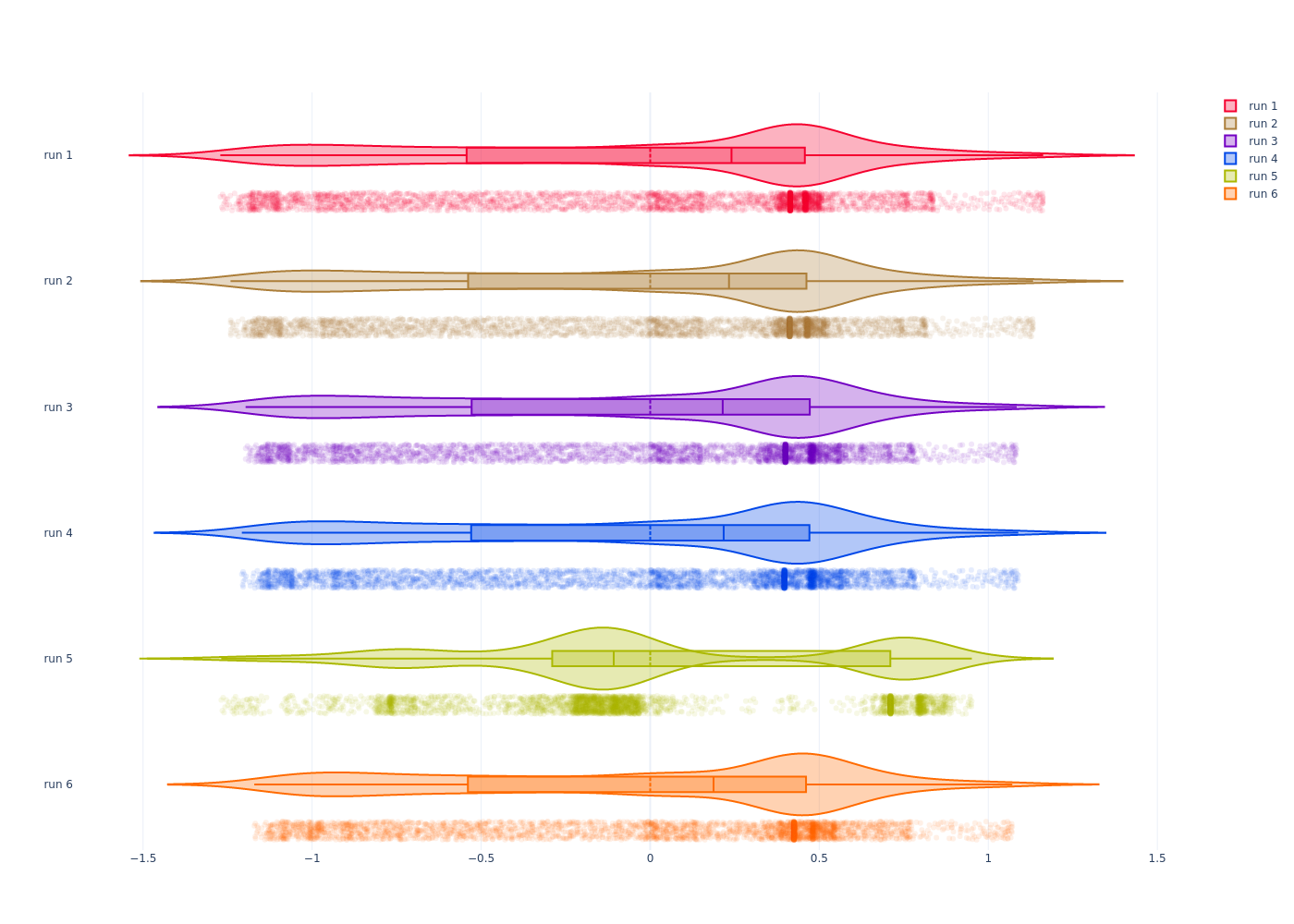
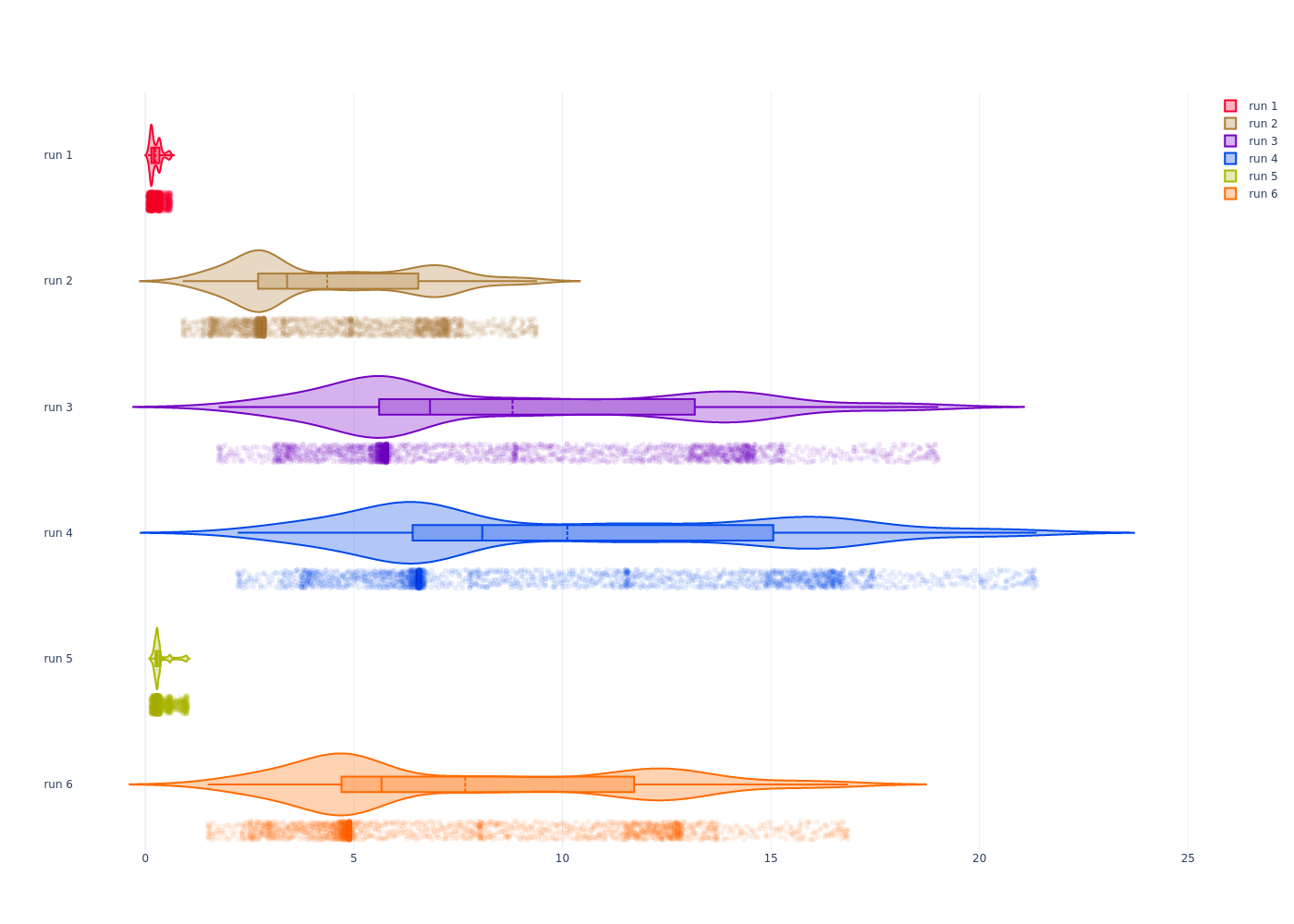
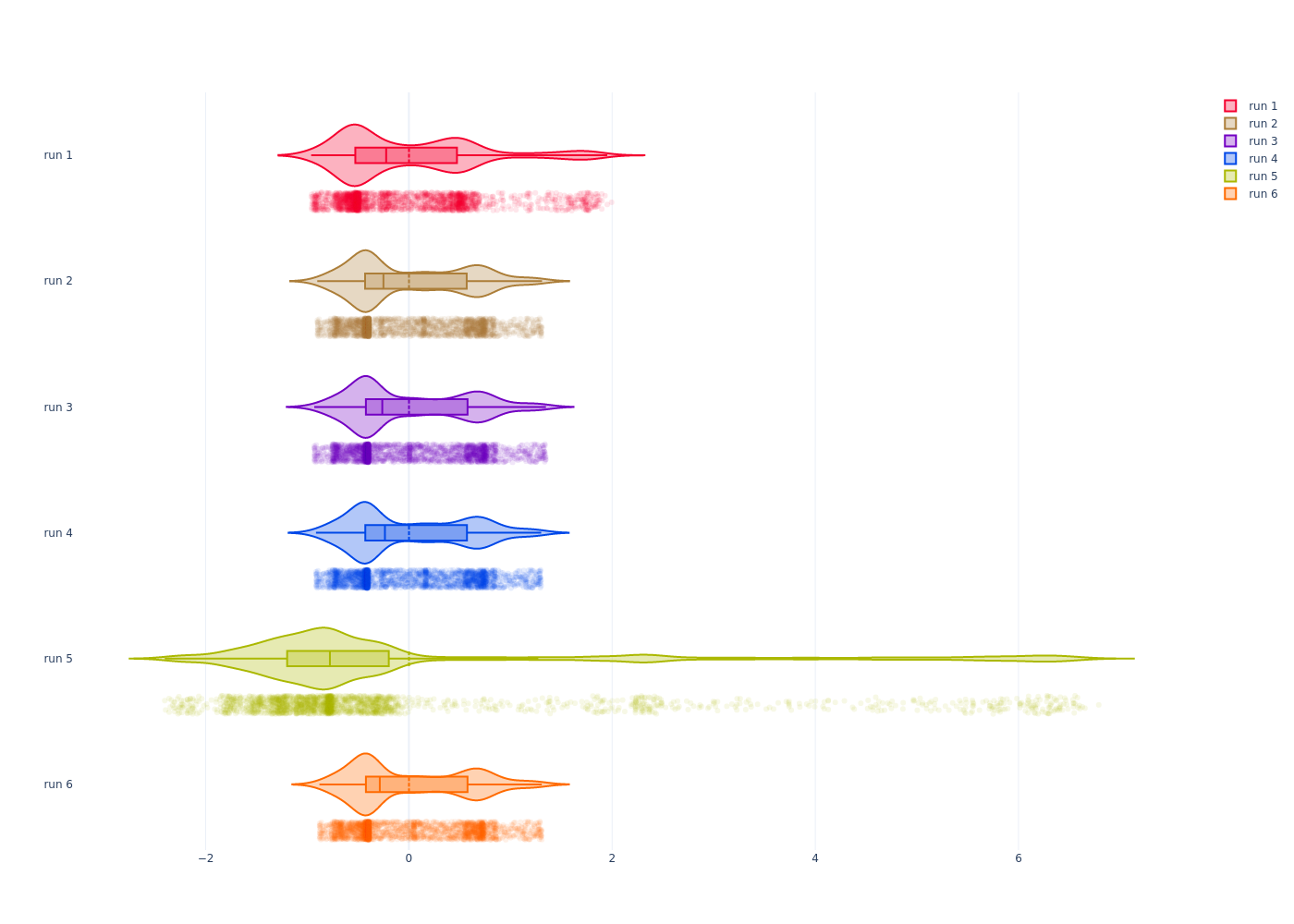
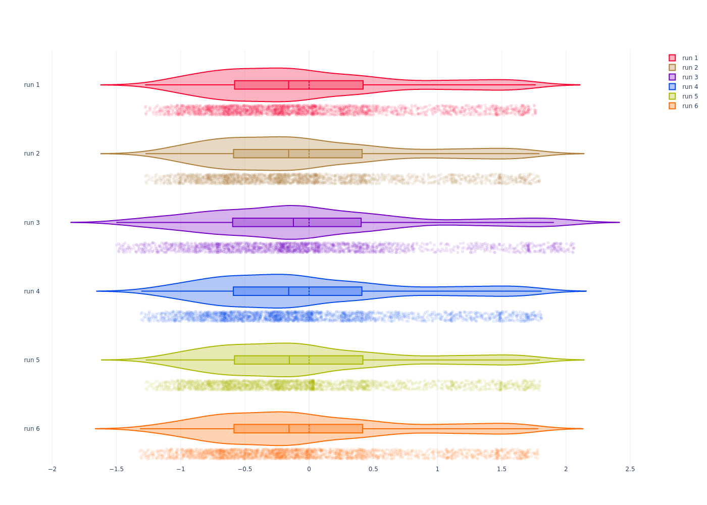
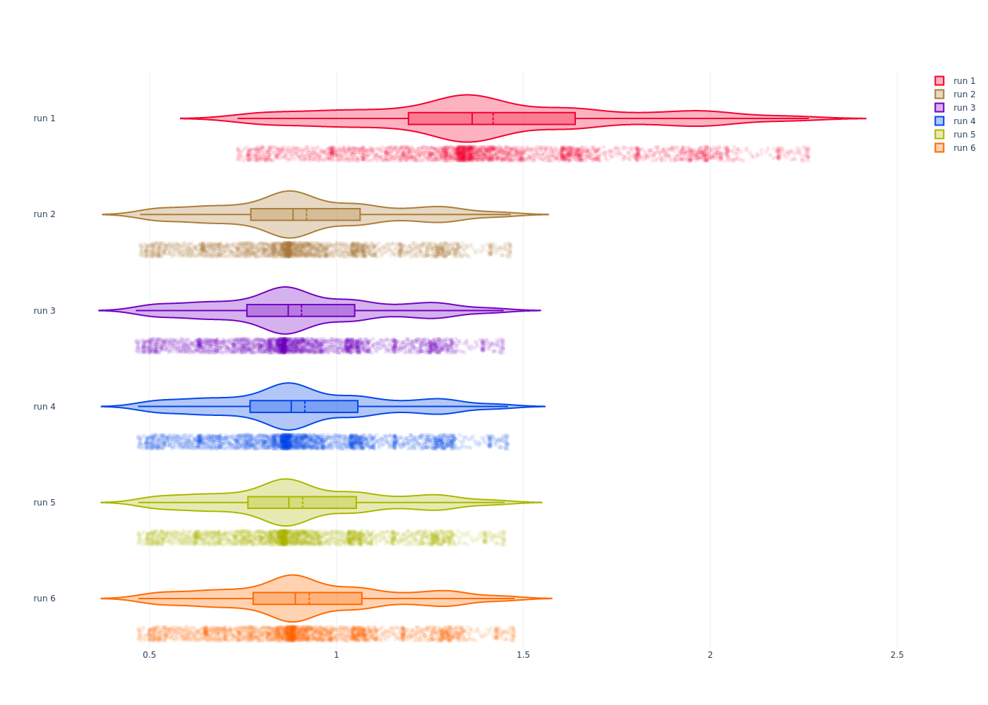
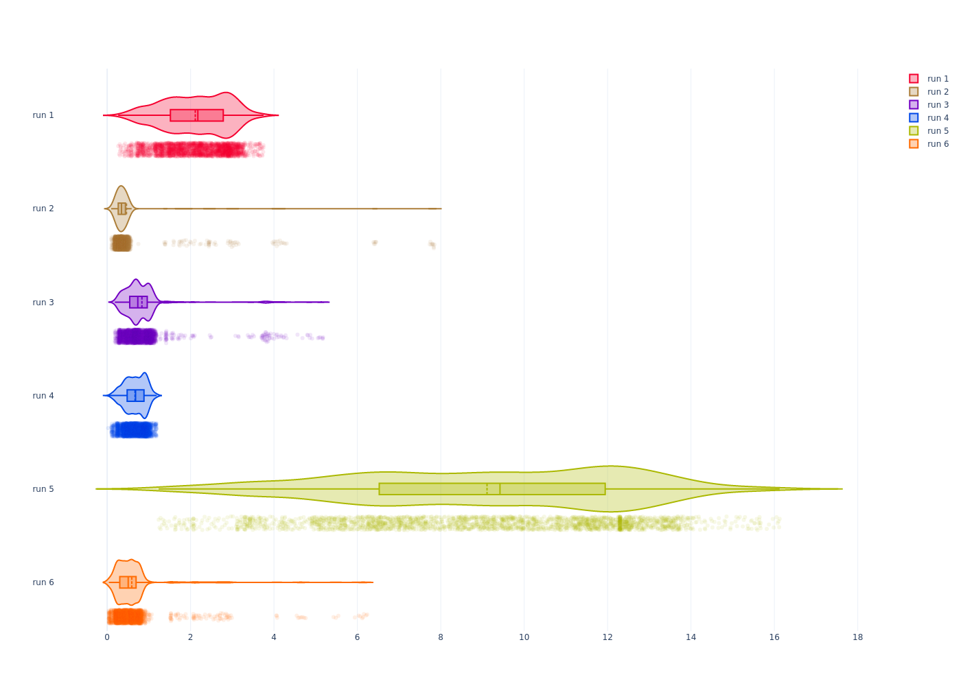
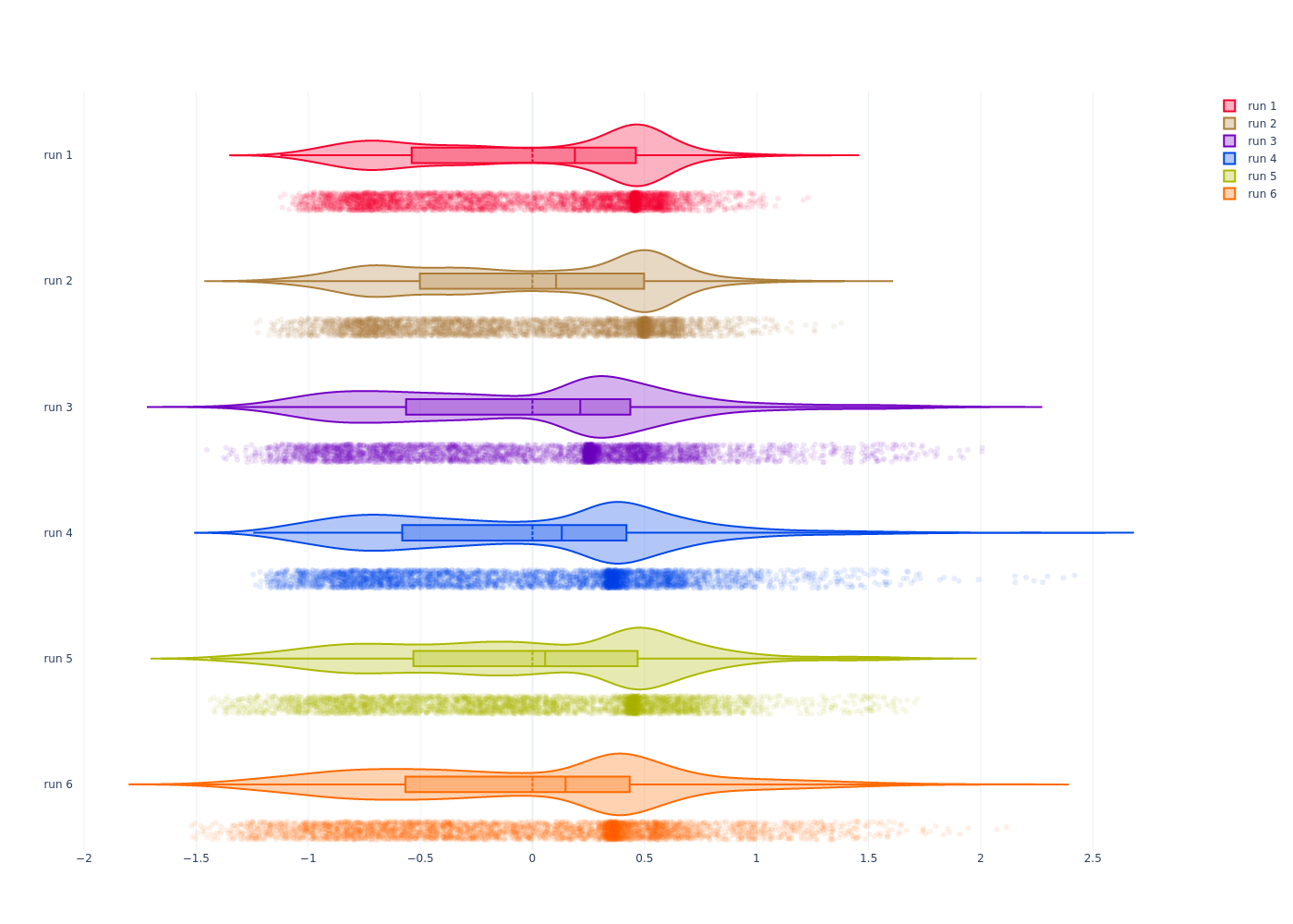
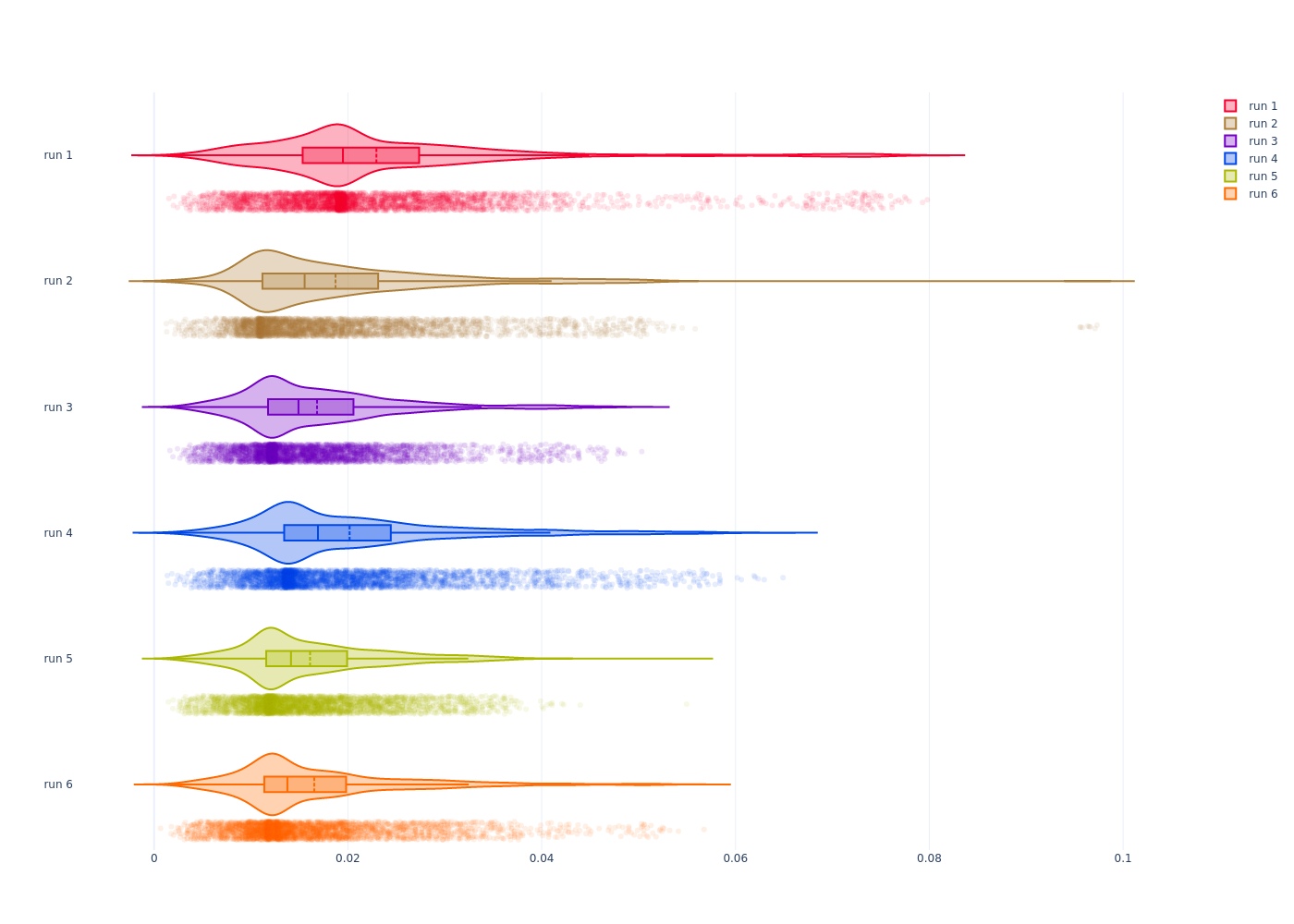
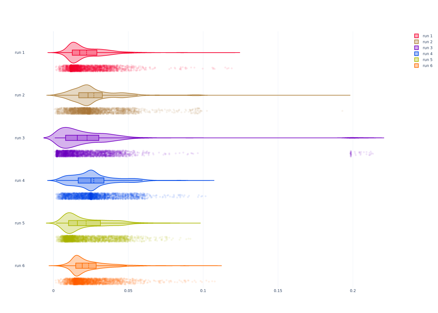
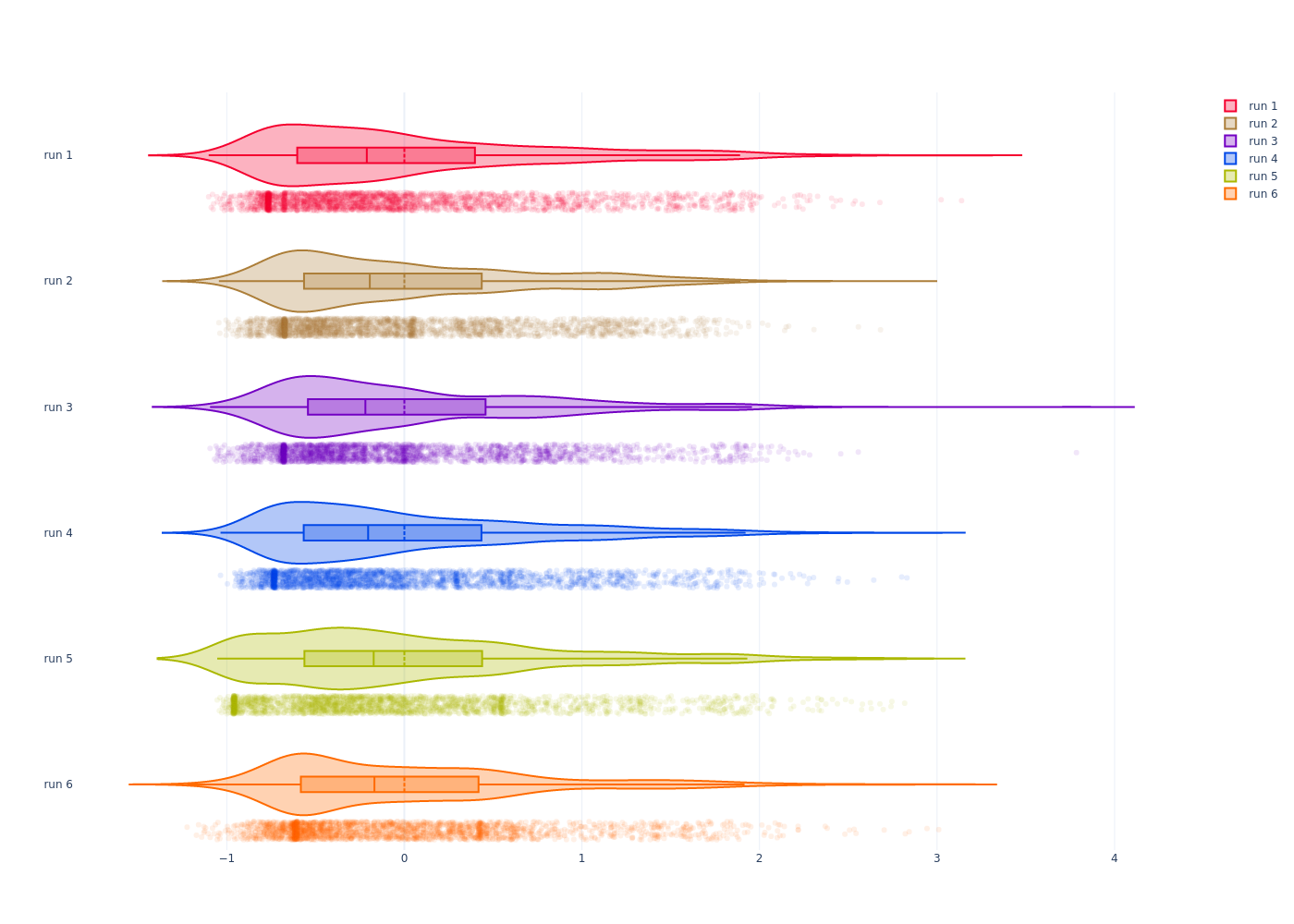
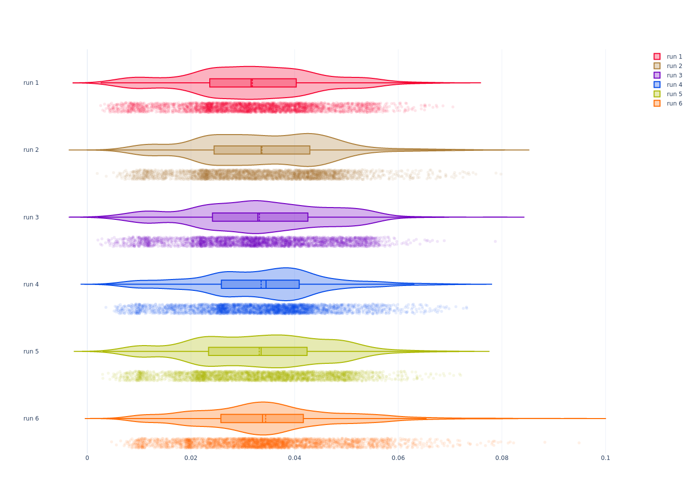
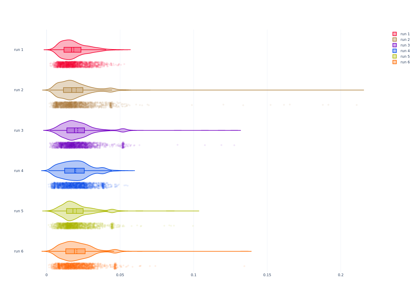
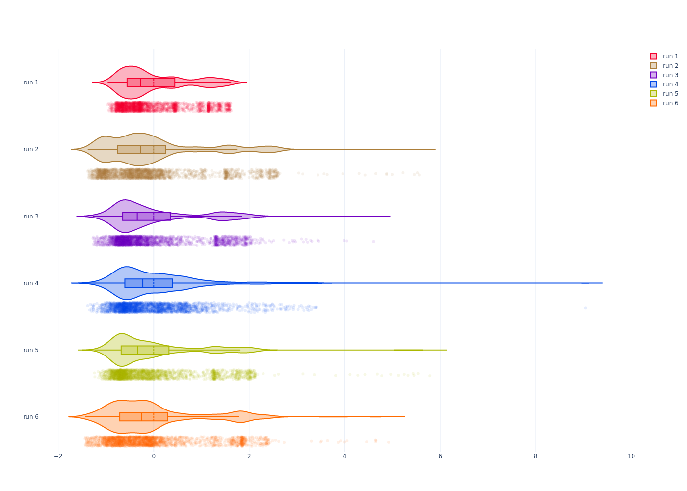
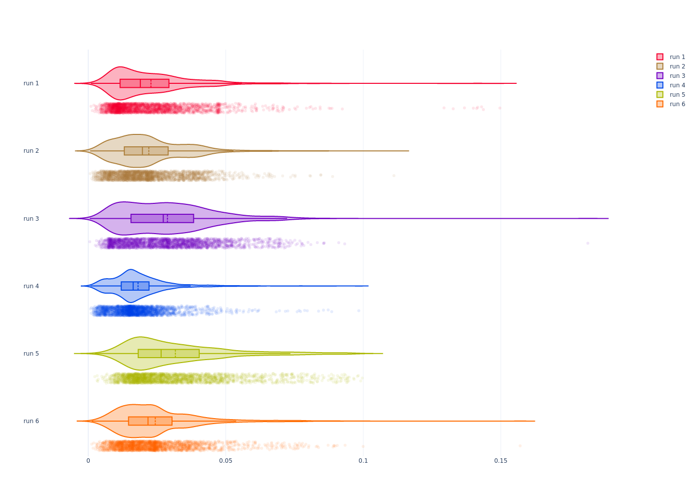
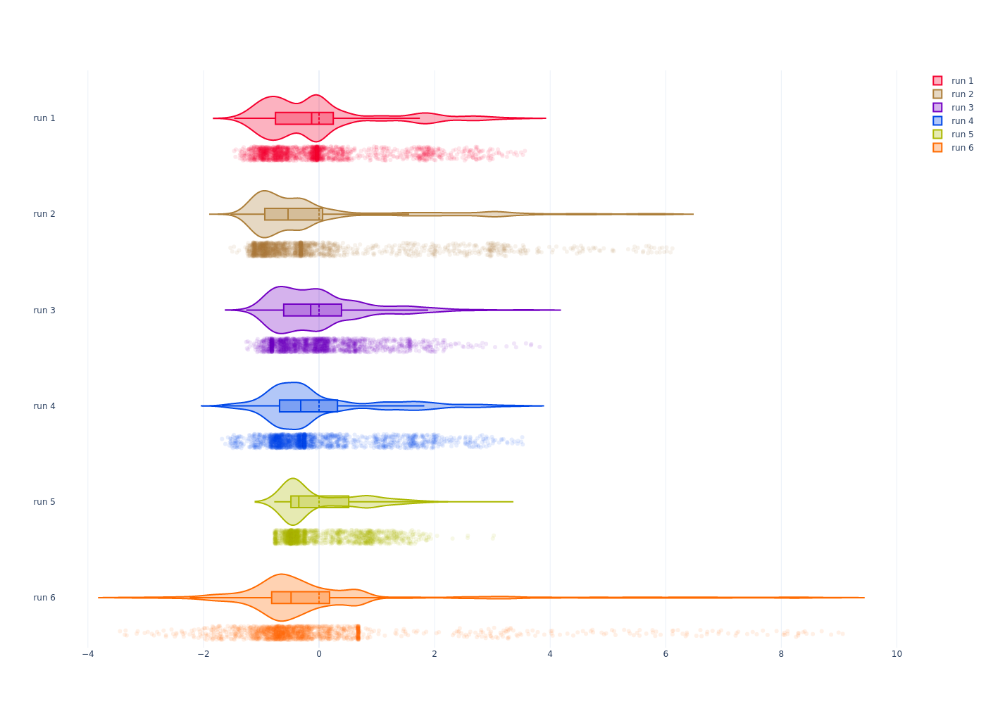
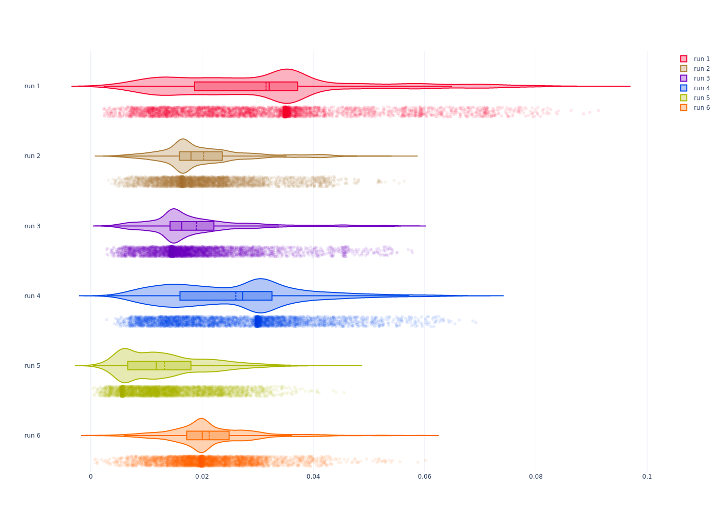
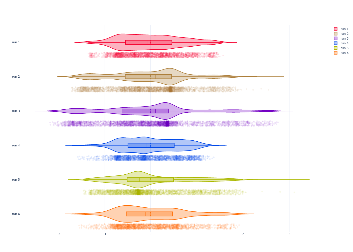
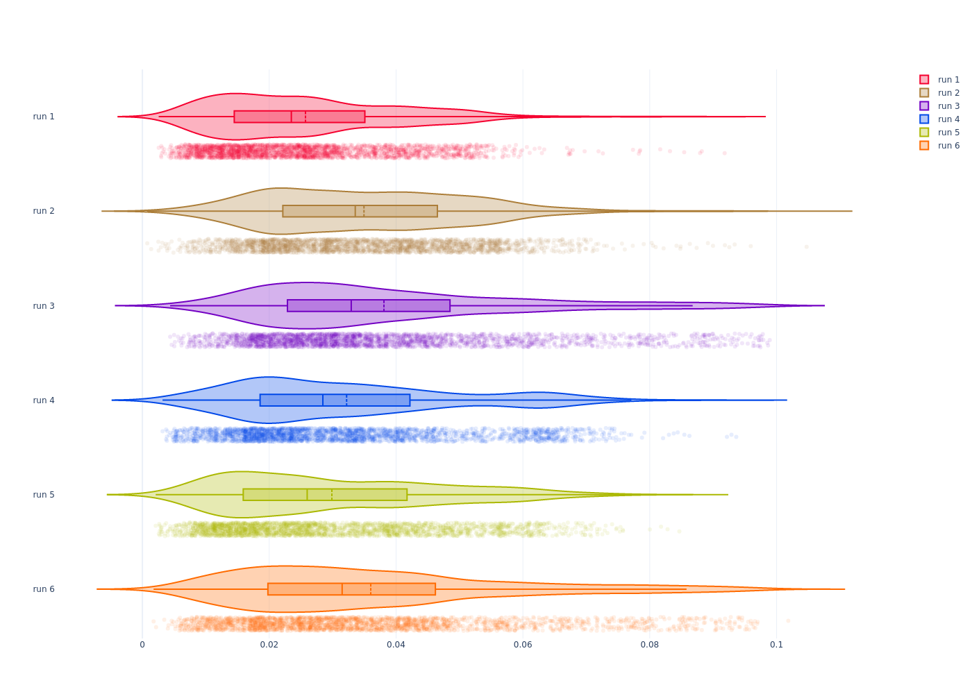
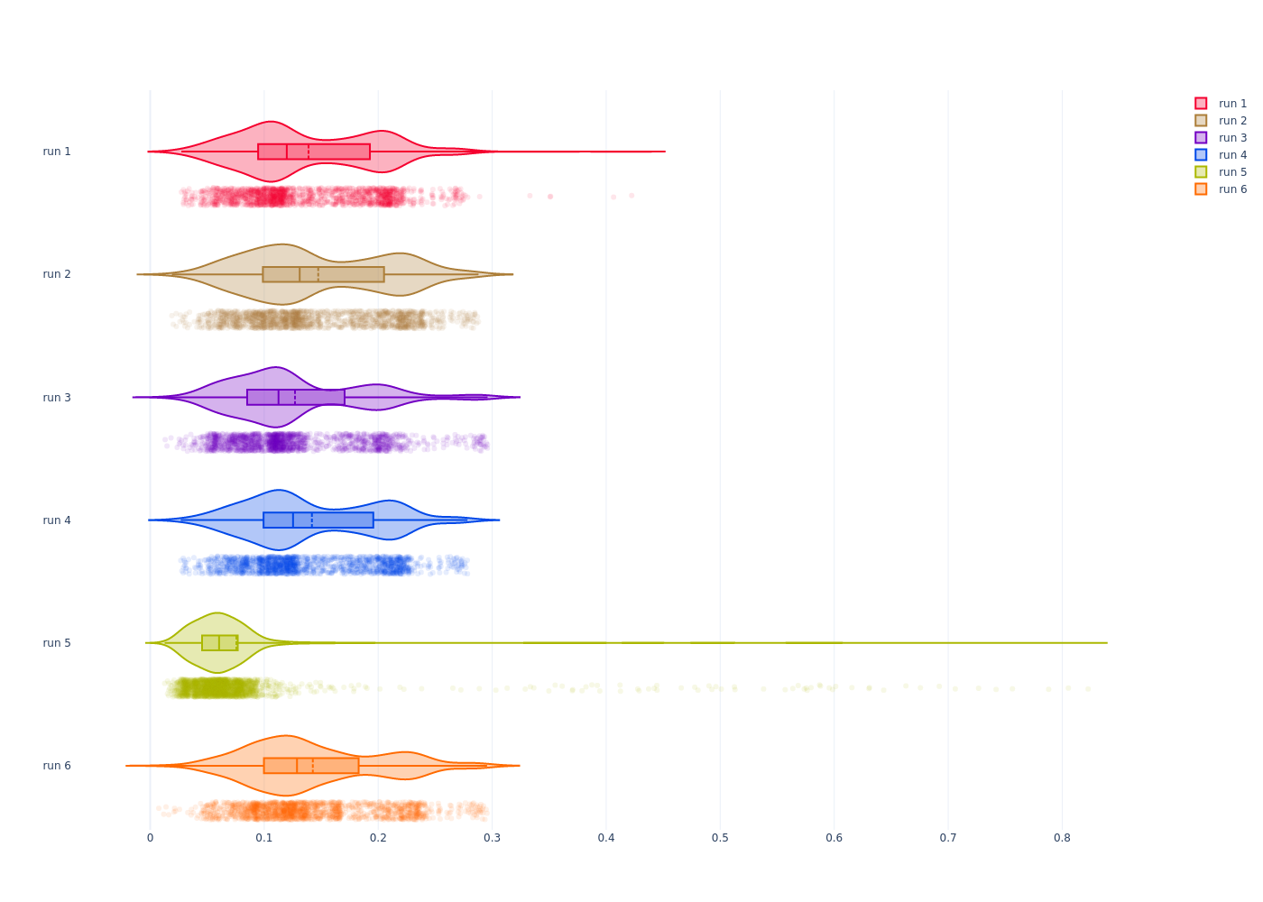
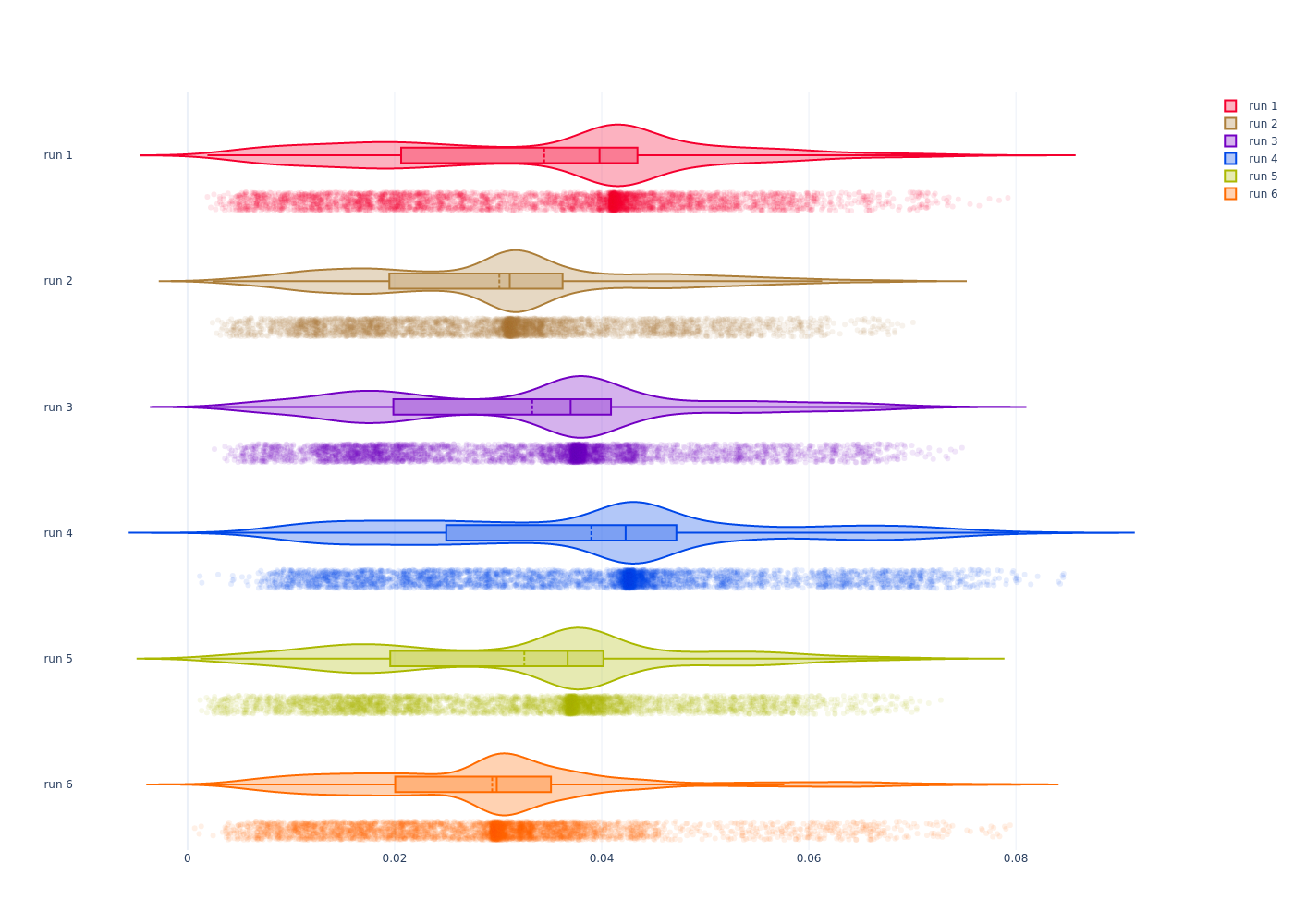
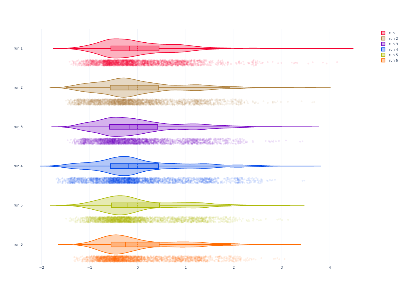
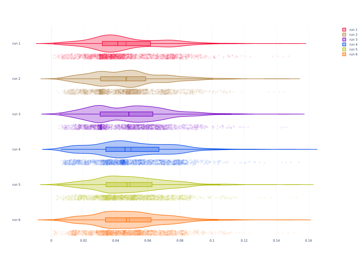
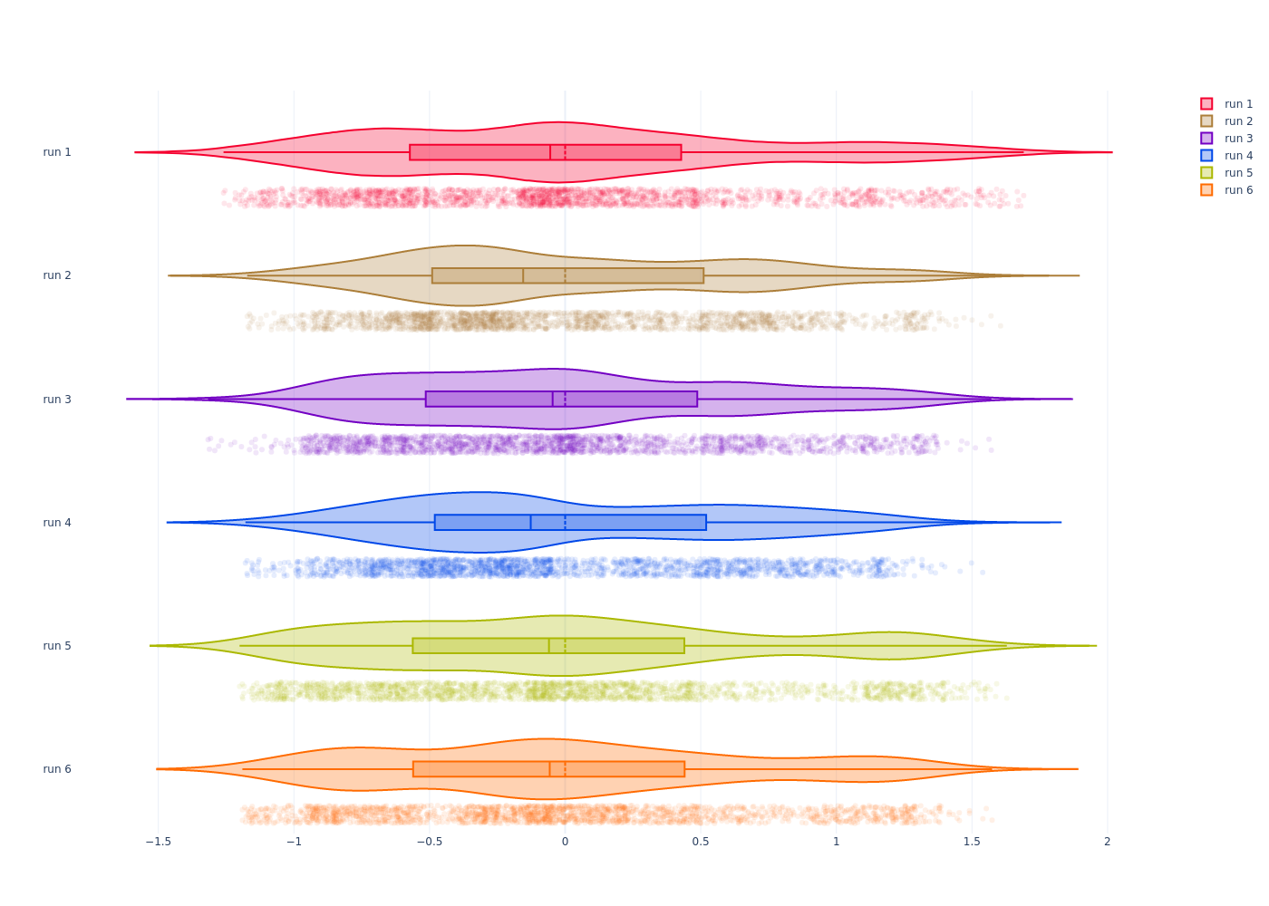
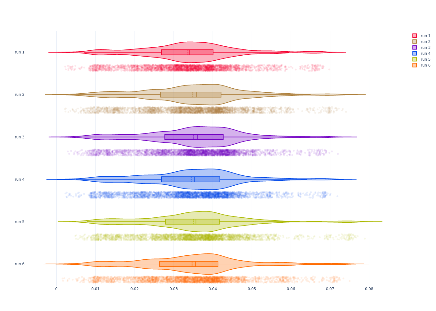
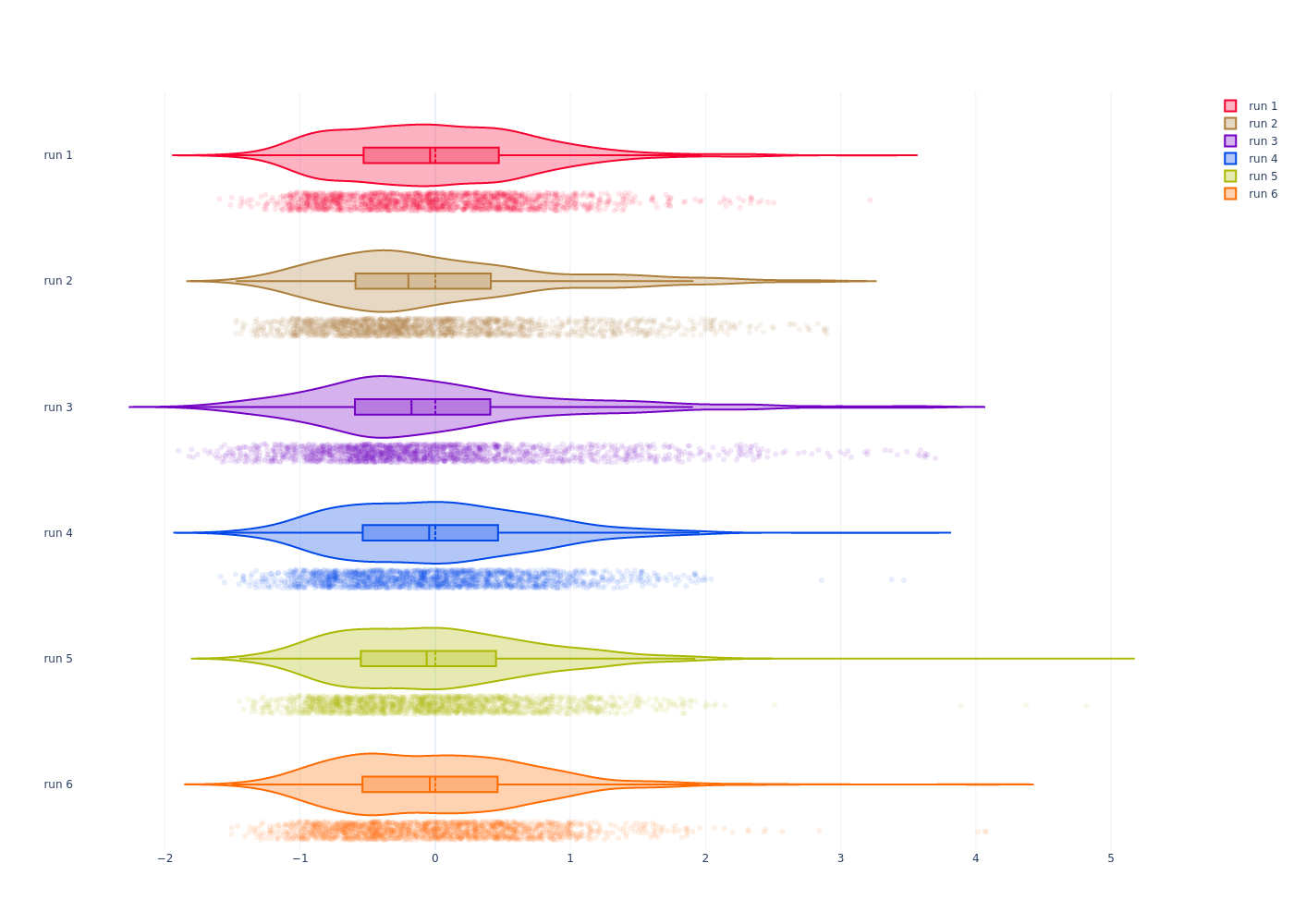
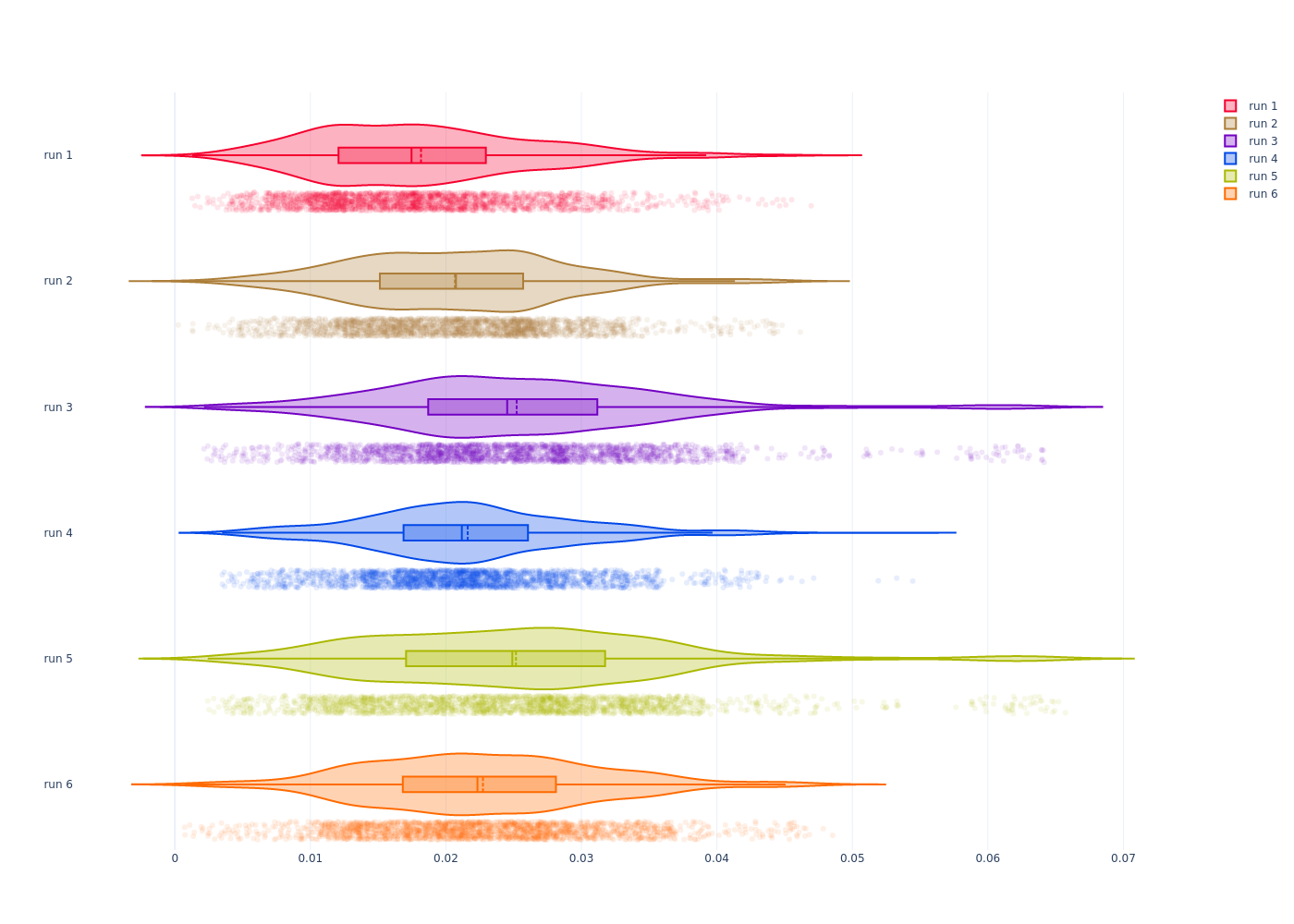
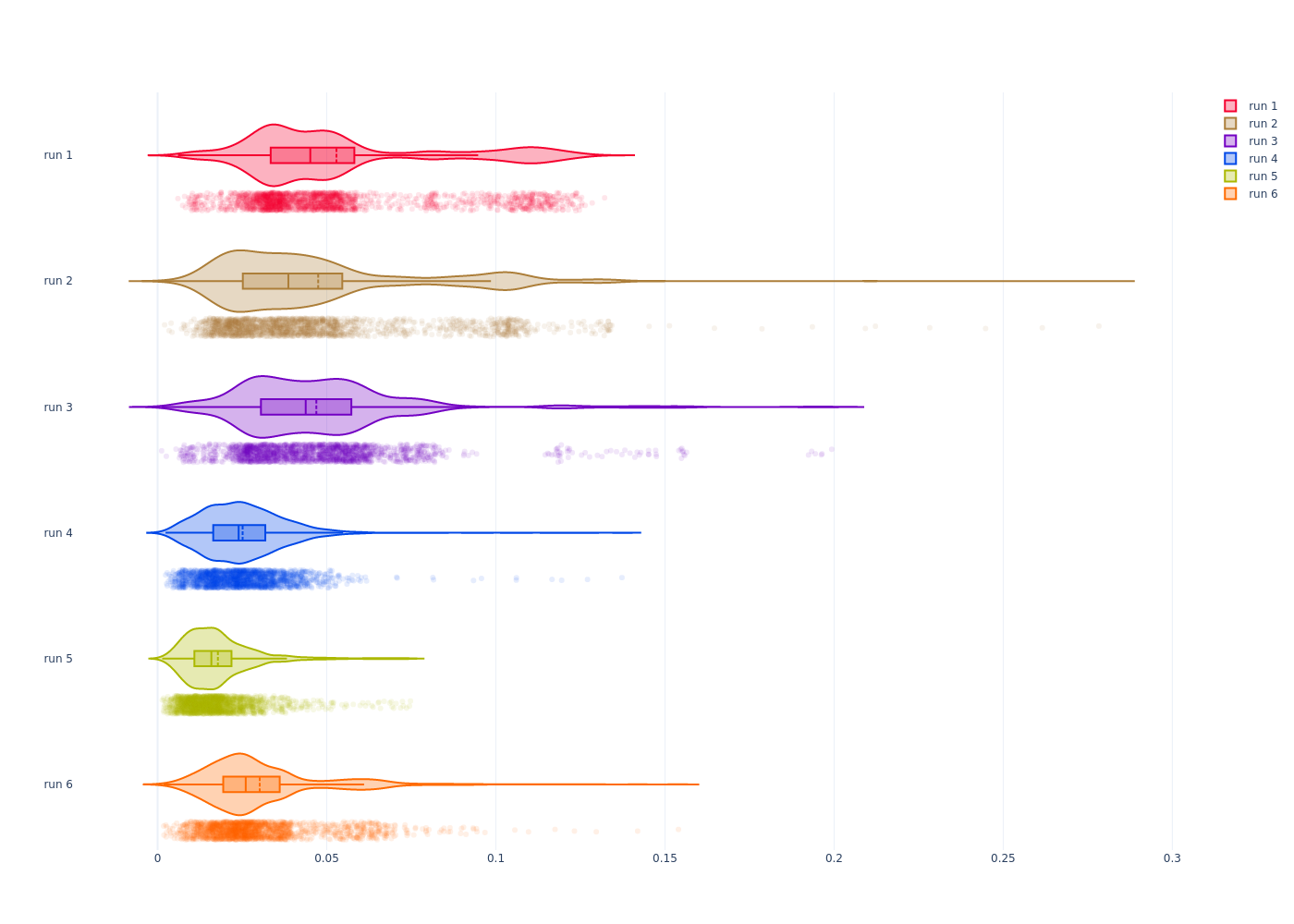
Violin plot, showing the error distributions for monocular runs 1 through 6 for the EuRoC MH02 dataset. Left: not normalized. Right: each run is normalized by its interquartile range, and its mean is set to 0.
Mann-Whitney U test
| run 1 | run 2 | run 3 | run 4 | run 5 | run 6 | |
|---|---|---|---|---|---|---|
| run 1 | 0.999994 | 0.000463474 | 0 | 0 | 8.57113e-168 | 0 |
| run 2 | 0.000463474 | 0.999994 | 0 | 0 | 4.20041e-174 | 0 |
| run 3 | 0 | 0 | 0.999994 | 9.24436e-134 | 0 | 0 |
| run 4 | 0 | 0 | 9.24436e-134 | 0.999994 | 0 | 0 |
| run 5 | 8.57113e-168 | 4.20041e-174 | 0 | 0 | 0.999994 | 0 |
| run 6 | 0 | 0 | 0 | 0 | 0 | 0.986745 |
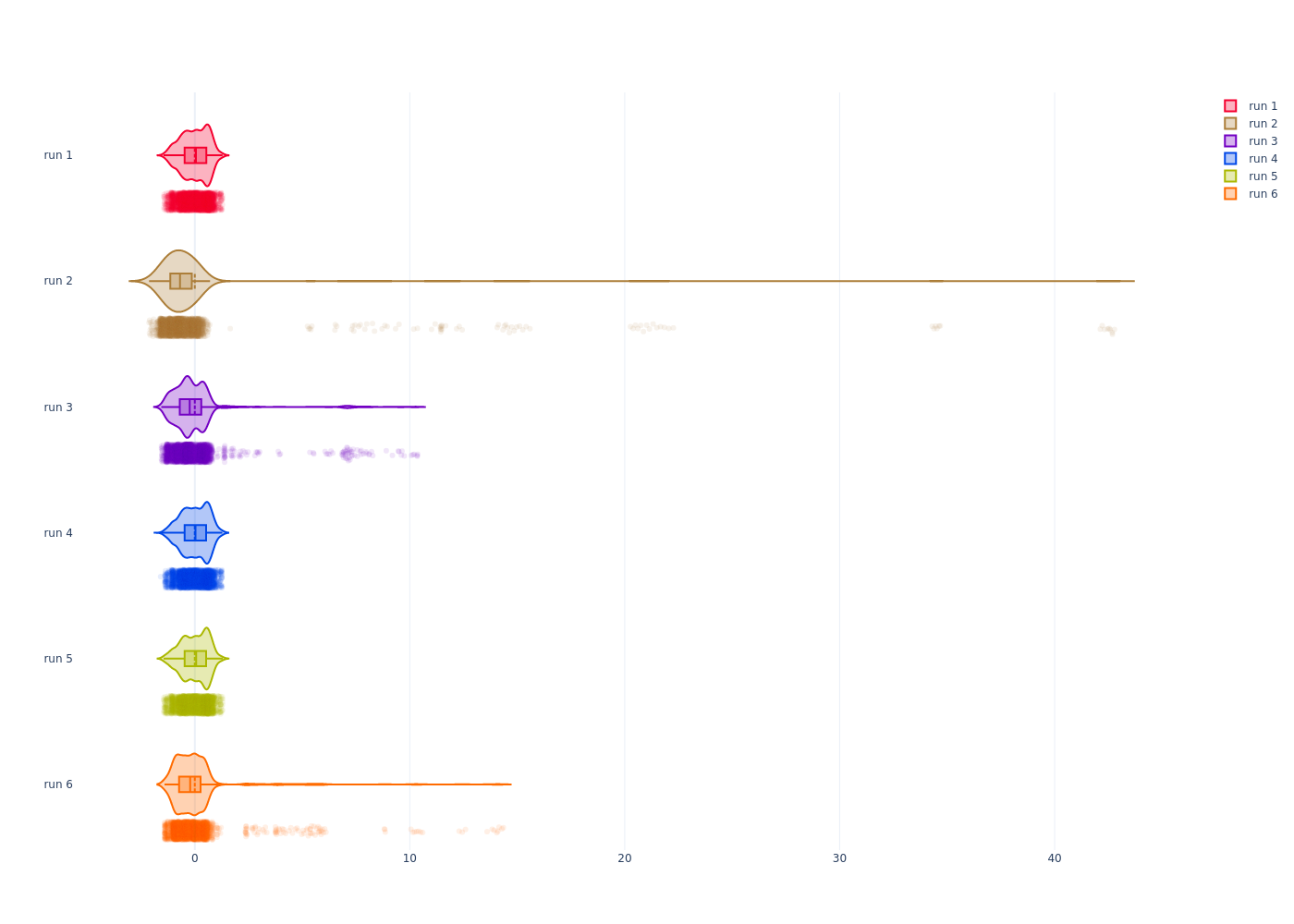
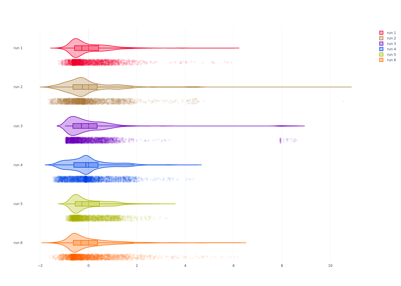
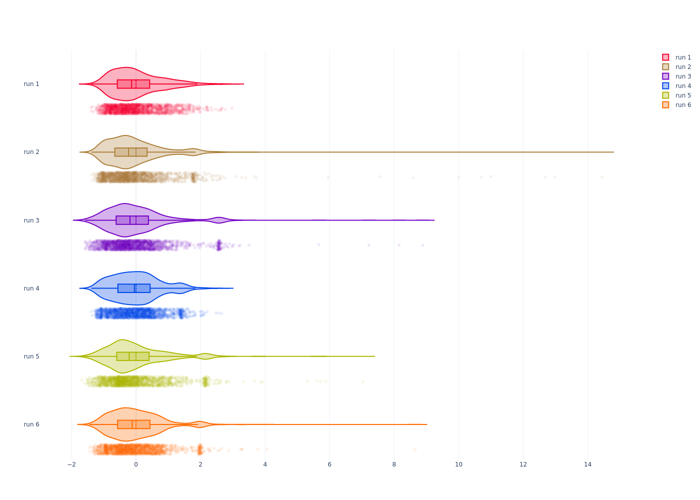
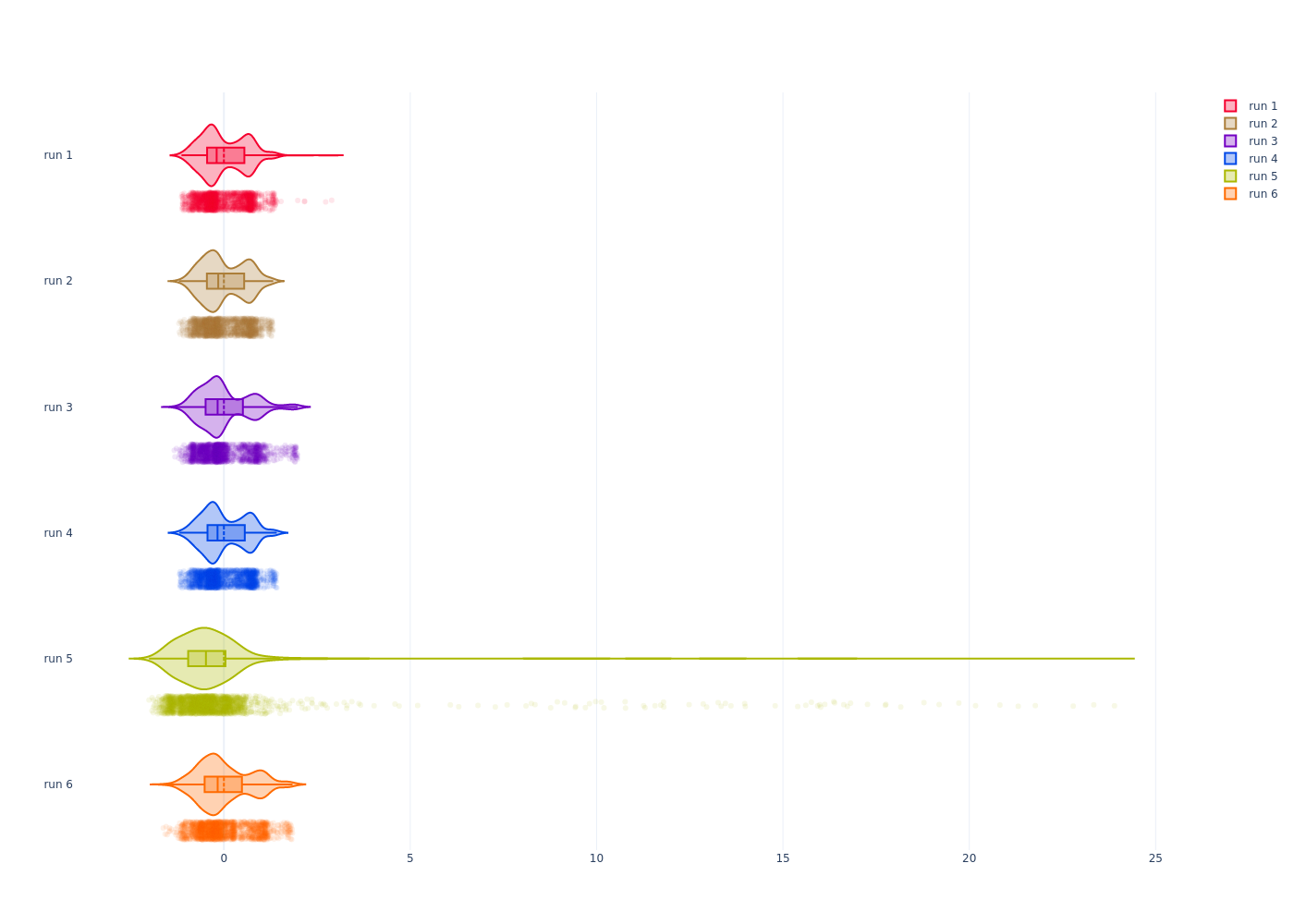
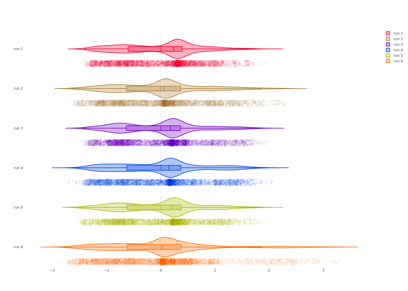
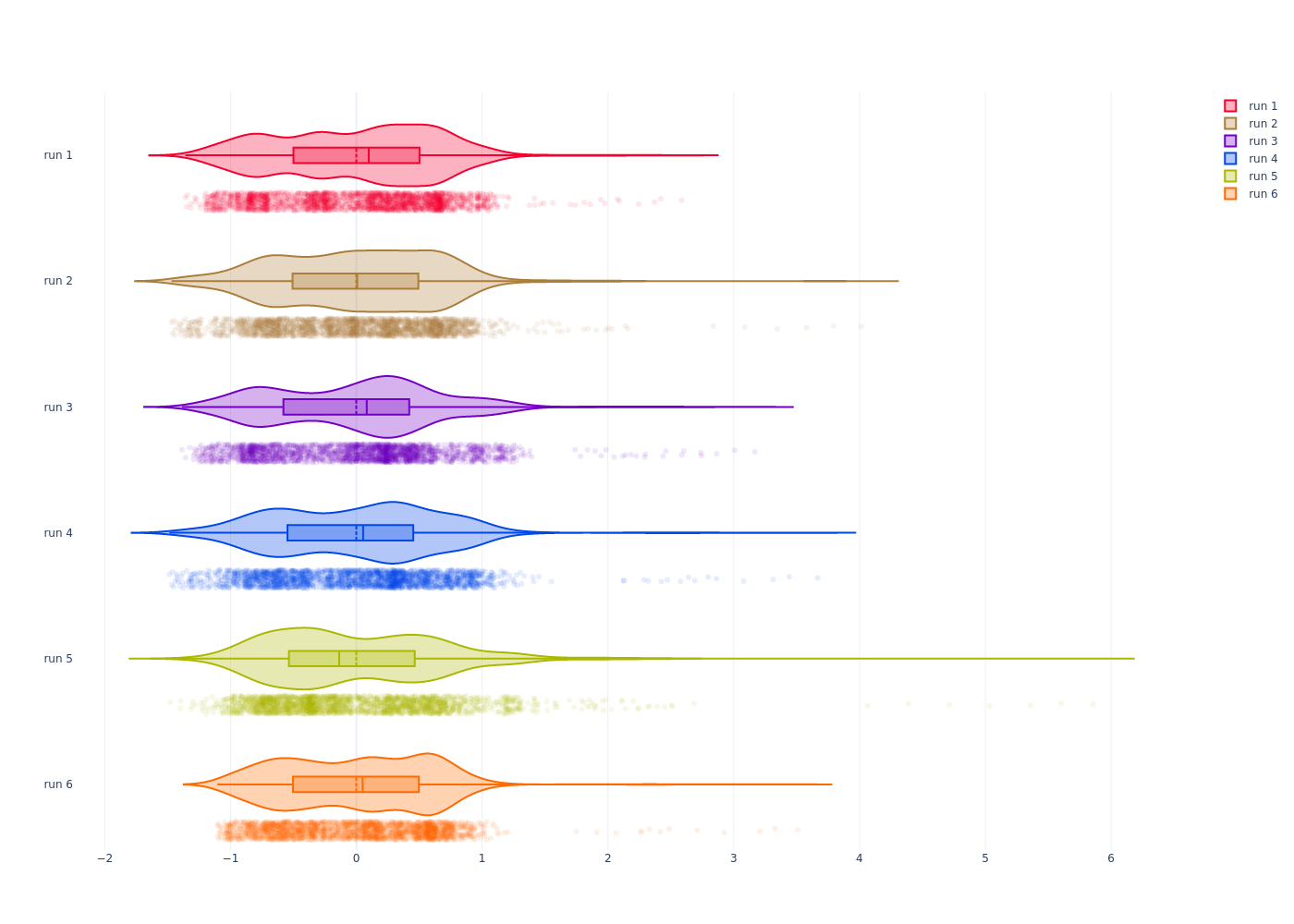
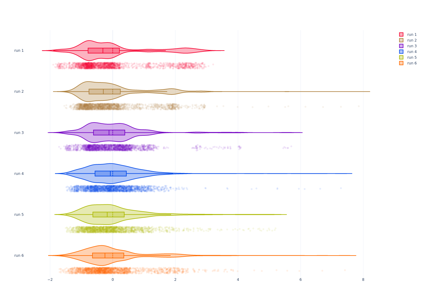
Violin plot, showing the error distributions for monocular runs 1 through 6 for the EuRoC MH03 dataset. Left: not normalized. Right: each run is normalized by its interquartile range, and its mean is set to 0.
Mann-Whitney U test
| run 1 | run 2 | run 3 | run 4 | run 5 | run 6 | |
|---|---|---|---|---|---|---|
| run 1 | 0.99697 | 0 | 0 | 0 | 0 | 0 |
| run 2 | 0 | 0.999985 | 0 | 0 | 0 | 0 |
| run 3 | 0 | 0 | 0.999978 | 0 | 0 | 3.06155e-188 |
| run 4 | 0 | 0 | 0 | 0.999993 | 0 | 0 |
| run 5 | 0 | 0 | 0 | 0 | 1 | 3.74558e-188 |
| run 6 | 0 | 0 | 3.06482e-188 | 0 | 3.74358e-188 | 1 |
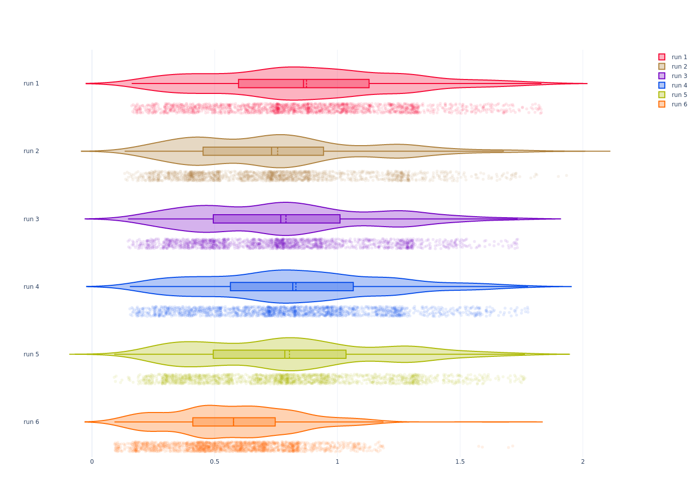
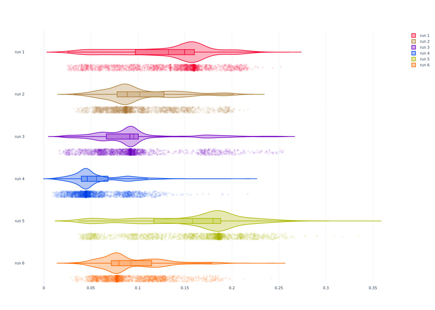
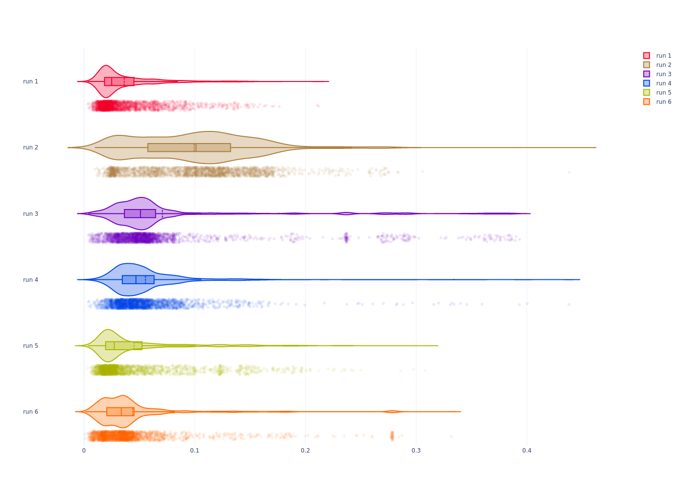
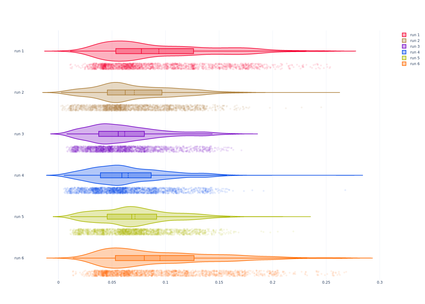
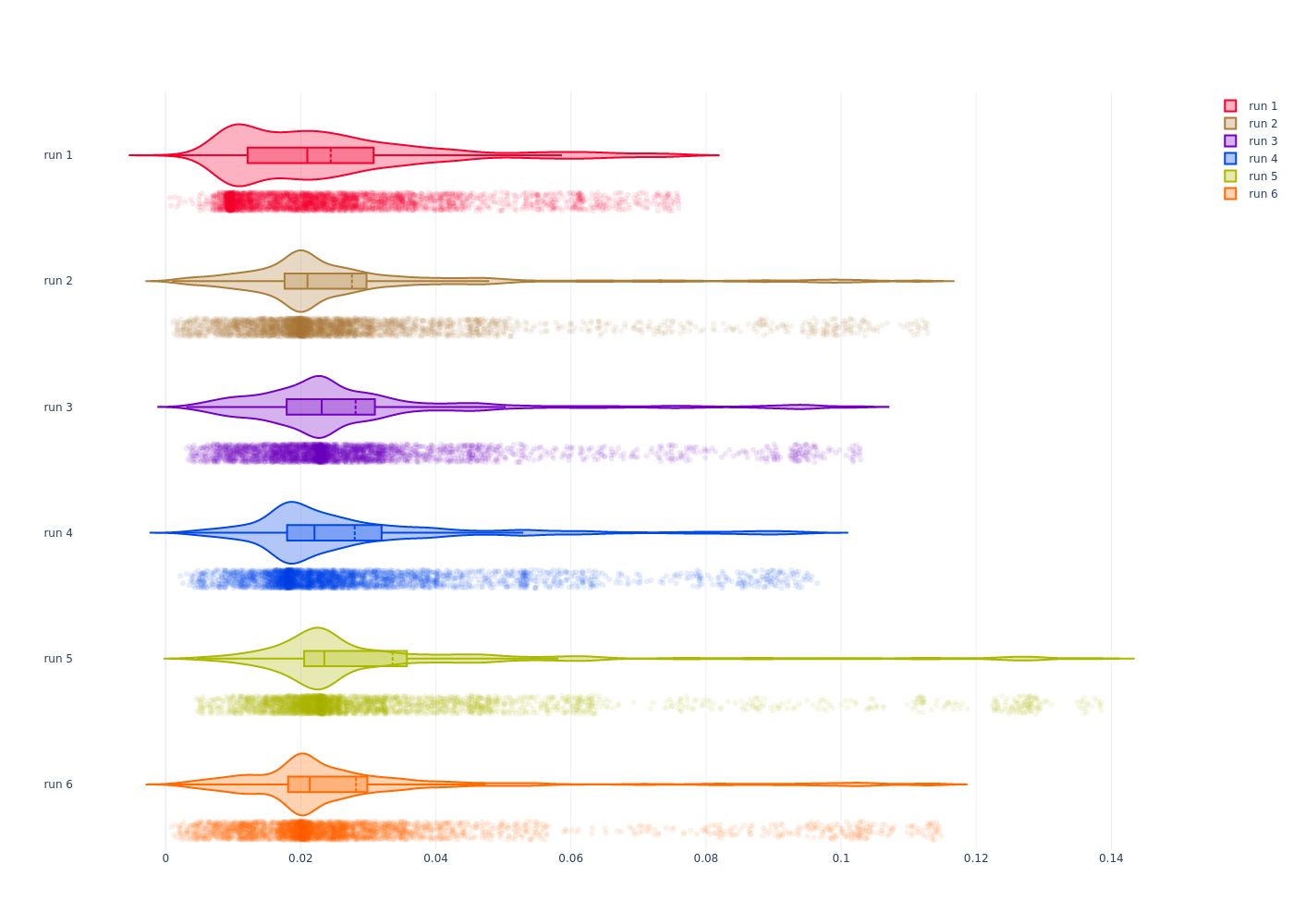
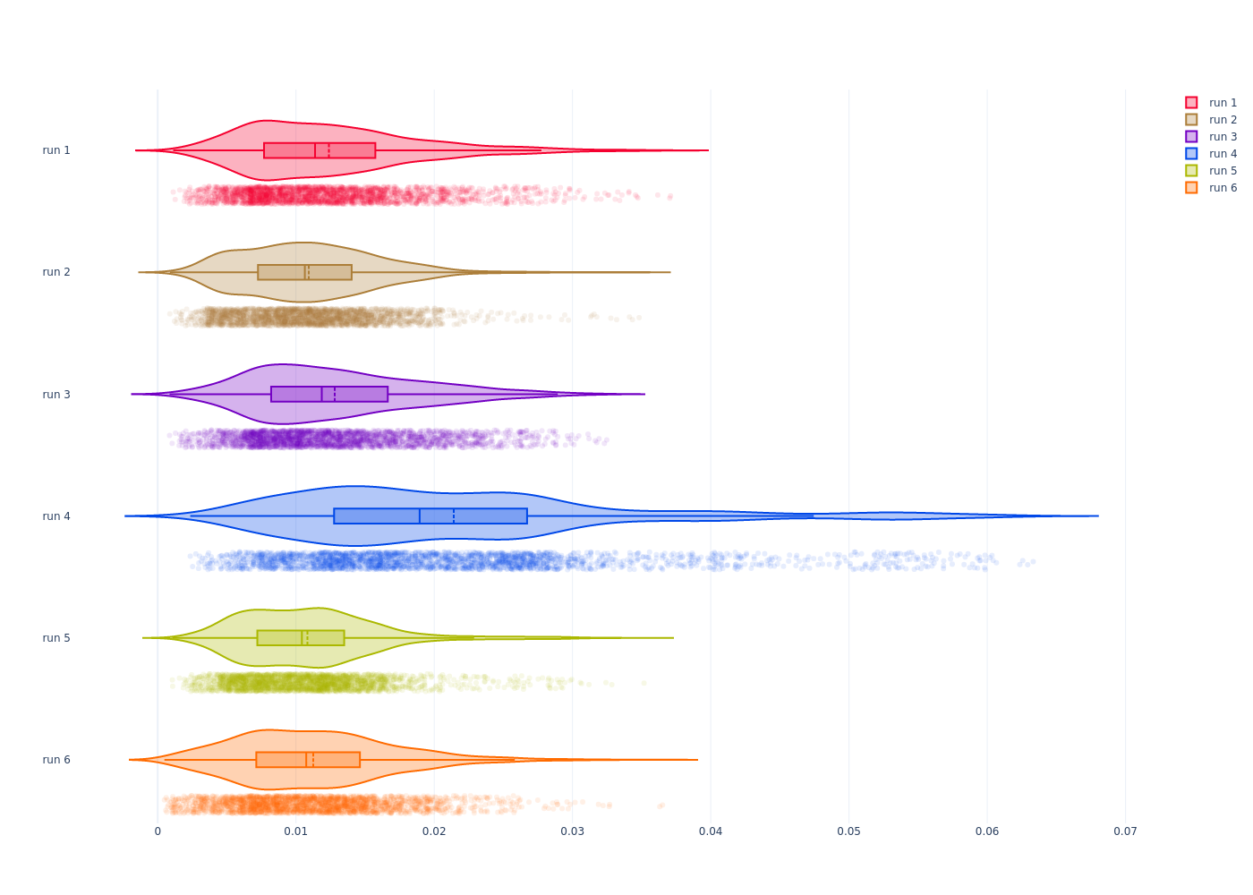
Violin plot, showing the error distributions for monocular runs 1 through 6 for the EuRoC MH04 dataset. Left: not normalized. Right: each run is normalized by its interquartile range, and its mean is set to 0.
Mann-Whitney U test
| run 1 | run 2 | run 3 | run 4 | run 5 | run 6 | |
|---|---|---|---|---|---|---|
| run 1 | 0.999508 | 0 | 0 | 0 | 7.67054e-92 | 0 |
| run 2 | 0 | 0.999989 | 3.48472e-235 | 6.40351e-302 | 0 | 6.30322e-156 |
| run 3 | 0 | 3.48472e-235 | 0.999877 | 1.19914e-26 | 0 | 2.67184e-30 |
| run 4 | 0 | 6.40351e-302 | 1.2064e-26 | 0.999654 | 0 | 2.43666e-67 |
| run 5 | 7.7409e-92 | 0 | 0 | 0 | 0.999955 | 0 |
| run 6 | 0 | 6.30322e-156 | 2.67184e-30 | 2.43666e-67 | 0 | 0.999989 |
Violin plot, showing the error distributions for monocular runs 1 through 6 for the EuRoC MH05 dataset. Left: not normalized. Right: each run is normalized by its interquartile range, and its mean is set to 0.
Mann-Whitney U test
| run 1 | run 2 | run 3 | run 4 | run 5 | run 6 | |
|---|---|---|---|---|---|---|
| run 1 | 0.999807 | 0 | 0 | 0 | 0 | 0 |
| run 2 | 0 | 0.999894 | 2.80229e-145 | 2.97841e-125 | 1.935e-129 | 8.13387e-306 |
| run 3 | 0 | 2.8163e-145 | 0.999961 | 1.01857e-05 | 0 | 7.75894e-60 |
| run 4 | 0 | 2.99222e-125 | 1.018e-05 | 0.999961 | 0 | 1.2426e-73 |
| run 5 | 0 | 1.93956e-129 | 0 | 0 | 1 | 0 |
| run 6 | 0 | 8.13387e-306 | 7.75894e-60 | 1.2426e-73 | 0 | 0.99999 |

Violin plot, showing the error distributions for monocular runs 1 through 6 for the EuRoC V101 dataset. Left: not normalized. Right: each run is normalized by its interquartile range, and its mean is set to 0.
Mann-Whitney U test
| run 1 | run 2 | run 3 | run 4 | run 5 | run 6 | |
|---|---|---|---|---|---|---|
| run 1 | 1 | 0.240639 | 0.837128 | 0.745791 | 0.634655 | 0.286821 |
| run 2 | 0.240639 | 0.999993 | 0.317526 | 0.373494 | 0.10581 | 0.898643 |
| run 3 | 0.837141 | 0.317526 | 1 | 0.89316 | 0.505919 | 0.372643 |
| run 4 | 0.745804 | 0.373494 | 0.893173 | 1 | 0.43212 | 0.43701 |
| run 5 | 0.634595 | 0.10581 | 0.505865 | 0.432072 | 0.999793 | 0.130874 |
| run 6 | 0.286836 | 0.898643 | 0.37266 | 0.43703 | 0.130874 | 0.999987 |
Violin plot, showing the error distributions for monocular runs 1 through 6 for the EuRoC V102 dataset. Left: not normalized. Right: each run is normalized by its interquartile range, and its mean is set to 0.
Mann-Whitney U test
| run 1 | run 2 | run 3 | run 4 | run 5 | run 6 | |
|---|---|---|---|---|---|---|
| run 1 | 0.999985 | 1.91394e-149 | 9.3959e-114 | 3.51903e-247 | 1.72768e-17 | 7.22398e-05 |
| run 2 | 1.91394e-149 | 0.974989 | 3.05152e-06 | 1.69562e-28 | 5.32088e-83 | 2.27054e-107 |
| run 3 | 9.3959e-114 | 3.06405e-06 | 1 | 3.89551e-56 | 2.45859e-54 | 2.53823e-77 |
| run 4 | 3.51903e-247 | 1.71604e-28 | 3.88842e-56 | 0.999985 | 3.9304e-177 | 7.67267e-195 |
| run 5 | 1.72768e-17 | 5.313e-83 | 2.46153e-54 | 3.93896e-177 | 0.999969 | 1.14773e-05 |
| run 6 | 7.22398e-05 | 4.71738e-108 | 2.584e-77 | 7.40583e-195 | 1.14733e-05 | 0.967018 |
Violin plot, showing the error distributions for monocular runs 1 through 6 for the EuRoC V103 dataset. Left: not normalized. Right: each run is normalized by its interquartile range, and its mean is set to 0.
Mann-Whitney U test
| run 1 | run 2 | run 3 | run 4 | run 5 | run 6 | |
|---|---|---|---|---|---|---|
| run 1 | 0.999654 | 6.19872e-25 | 1.21581e-95 | 6.34245e-07 | 4.83033e-11 | 0.000276094 |
| run 2 | 6.36126e-25 | 0.99068 | 3.66909e-32 | 6.02063e-08 | 2.29596e-05 | 1.53756e-38 |
| run 3 | 2.01536e-95 | 1.90032e-31 | 0.403558 | 9.47975e-59 | 2.97185e-55 | 5.60843e-114 |
| run 4 | 6.57073e-07 | 4.74874e-08 | 6.69292e-61 | 0.949662 | 0.0819202 | 5.34868e-16 |
| run 5 | 4.83033e-11 | 2.29596e-05 | 2.97185e-55 | 0.0819202 | 0.999989 | 1.94416e-22 |
| run 6 | 0.000268382 | 8.6962e-39 | 3.61242e-117 | 1.75719e-16 | 1.94416e-22 | 0.943499 |
Violin plot, showing the error distributions for monocular runs 1 through 6 for the EuRoC V201 dataset. Left: not normalized. Right: each run is normalized by its interquartile range, and its mean is set to 0.
Mann-Whitney U test
| run 1 | run 2 | run 3 | run 4 | run 5 | run 6 | |
|---|---|---|---|---|---|---|
| run 1 | 0.99999 | 0 | 0 | 0 | 0 | 0 |
| run 2 | 0 | 1 | 0.0198496 | 0.446756 | 0.0541684 | 0.134809 |
| run 3 | 0 | 0.0198523 | 0.999969 | 0.093686 | 0.658669 | 0.000346848 |
| run 4 | 0 | 0.446787 | 0.0936657 | 0.999979 | 0.205632 | 0.0303575 |
| run 5 | 0 | 0.0541748 | 0.658594 | 0.20566 | 0.999979 | 0.00139763 |
| run 6 | 0 | 0.134795 | 0.000346711 | 0.0303496 | 0.00139713 | 0.999969 |
Violin plot, showing the error distributions for monocular runs 1 through 6 for the EuRoC V202 dataset. Left: not normalized. Right: each run is normalized by its interquartile range, and its mean is set to 0.
Mann-Whitney U test
| run 1 | run 2 | run 3 | run 4 | run 5 | run 6 | |
|---|---|---|---|---|---|---|
| run 1 | 0.980484 | 0 | 0 | 0 | 0 | 0 |
| run 2 | 0 | 0.914929 | 0 | 1.86581e-277 | 0 | 3.97714e-85 |
| run 3 | 0 | 0 | 0.914929 | 2.27896e-21 | 0 | 3.02748e-132 |
| run 4 | 0 | 5.1506e-276 | 9.27289e-22 | 0.9763 | 0 | 2.64718e-71 |
| run 5 | 0 | 0 | 0 | 0 | 0.999991 | 0 |
| run 6 | 0 | 1.54233e-83 | 3.00283e-134 | 5.42453e-72 | 0 | 0.931306 |
Violin plot, showing the error distributions for monocular runs 1 through 6 for the EuRoC V203 dataset. Left: not normalized. Right: each run is normalized by its interquartile range, and its mean is set to 0.
Mann-Whitney U test
| run 1 | run 2 | run 3 | run 4 | run 5 | run 6 | |
|---|---|---|---|---|---|---|
| run 1 | 0.87569 | 5.0151e-10 | 1.78474e-07 | 0.000725441 | 3.15151e-09 | 8.75078e-132 |
| run 2 | 2.85472e-11 | 0.699751 | 0.0990505 | 0.000418325 | 0.405158 | 4.1184e-64 |
| run 3 | 2.7359e-08 | 0.244927 | 0.849464 | 0.0229335 | 0.66153 | 1.6587e-79 |
| run 4 | 0.000293474 | 0.00136482 | 0.0438792 | 0.916954 | 0.00661606 | 2.14917e-106 |
| run 5 | 1.24529e-09 | 0.520908 | 0.551473 | 0.00441163 | 0.96069 | 8.52124e-76 |
| run 6 | 8.75078e-132 | 4.1184e-64 | 1.6587e-79 | 2.14917e-106 | 8.52124e-76 | 0.999985 |
Stereo
Violin plot, showing the error distributions for stereo runs 1 through 6 for the EuRoC MH01 dataset. Left: not normalized. Right: each run is normalized by its interquartile range, and its mean is set to 0.
Mann-Whitney U test
| run 1 | run 2 | run 3 | run 4 | run 5 | run 6 | |
|---|---|---|---|---|---|---|
| run 1 | 0.999996 | 1.6325e-89 | 6.91828e-221 | 1.09163e-290 | 5.77401e-221 | 1.44596e-202 |
| run 2 | 1.6325e-89 | 0.999996 | 8.17437e-102 | 4.09189e-166 | 1.90661e-104 | 6.89817e-84 |
| run 3 | 6.91828e-221 | 8.17437e-102 | 0.999996 | 1.5707e-26 | 0.0426541 | 2.22768e-05 |
| run 4 | 1.09163e-290 | 4.09189e-166 | 1.5707e-26 | 0.999996 | 2.15172e-28 | 5.13282e-42 |
| run 5 | 5.77401e-221 | 1.90661e-104 | 0.0426541 | 2.15172e-28 | 0.999996 | 0.427157 |
| run 6 | 1.44596e-202 | 6.89817e-84 | 2.22768e-05 | 5.13282e-42 | 0.427157 | 0.999996 |
Violin plot, showing the error distributions for stereo runs 1 through 6 for the EuRoC MH02 dataset. Left: not normalized. Right: each run is normalized by its interquartile range, and its mean is set to 0.
Mann-Whitney U test
| run 1 | run 2 | run 3 | run 4 | run 5 | run 6 | |
|---|---|---|---|---|---|---|
| run 1 | 0.999994 | 5.43802e-59 | 2.99342e-108 | 5.39413e-24 | 6.97265e-135 | 1.89896e-130 |
| run 2 | 5.43802e-59 | 0.999994 | 1.14236e-05 | 2.87258e-14 | 9.07753e-12 | 1.02741e-12 |
| run 3 | 2.99342e-108 | 1.14236e-05 | 0.999994 | 6.25574e-38 | 0.00451676 | 0.00148004 |
| run 4 | 5.39413e-24 | 2.87258e-14 | 6.25574e-38 | 0.999994 | 2.58418e-55 | 1.81812e-56 |
| run 5 | 6.97265e-135 | 9.07753e-12 | 0.00451676 | 2.58418e-55 | 0.999994 | 0.662021 |
| run 6 | 1.89896e-130 | 1.02741e-12 | 0.00148004 | 1.81812e-56 | 0.662021 | 0.999994 |
Violin plot, showing the error distributions for stereo runs 1 through 6 for the EuRoC MH03 dataset. Left: not normalized. Right: each run is normalized by its interquartile range, and its mean is set to 0.
Mann-Whitney U test
| run 1 | run 2 | run 3 | run 4 | run 5 | run 6 | |
|---|---|---|---|---|---|---|
| run 1 | 0.999993 | 1.32769e-41 | 1.31444e-19 | 9.59055e-42 | 5.81017e-09 | 3.08343e-12 |
| run 2 | 1.32769e-41 | 0.999993 | 8.66529e-71 | 0.0138233 | 4.61542e-53 | 3.01353e-21 |
| run 3 | 1.31444e-19 | 8.66529e-71 | 0.999993 | 2.34469e-73 | 2.76581e-08 | 1.61587e-38 |
| run 4 | 9.59055e-42 | 0.0138233 | 2.34469e-73 | 0.999993 | 1.76406e-50 | 1.18388e-25 |
| run 5 | 5.81017e-09 | 4.61542e-53 | 2.76581e-08 | 1.76406e-50 | 0.999993 | 9.71456e-28 |
| run 6 | 3.08343e-12 | 3.01353e-21 | 1.61587e-38 | 1.18388e-25 | 9.71456e-28 | 0.999993 |
Violin plot, showing the error distributions for stereo runs 1 through 6 for the EuRoC MH04 dataset. Left: not normalized. Right: each run is normalized by its interquartile range, and its mean is set to 0.
Mann-Whitney U test
| run 1 | run 2 | run 3 | run 4 | run 5 | run 6 | |
|---|---|---|---|---|---|---|
| run 1 | 0.999989 | 1.65029e-103 | 7.39291e-119 | 0 | 9.34754e-75 | 5.84121e-160 |
| run 2 | 1.65029e-103 | 0.999989 | 4.26786e-07 | 0 | 1.03863e-212 | 9.02303e-22 |
| run 3 | 7.39291e-119 | 4.26786e-07 | 0.999989 | 3.20054e-226 | 1.67999e-228 | 0.229224 |
| run 4 | 0 | 0 | 3.20054e-226 | 0.999989 | 0 | 3.96237e-272 |
| run 5 | 9.34754e-75 | 1.03863e-212 | 1.67999e-228 | 0 | 0.999989 | 1.03536e-270 |
| run 6 | 5.84121e-160 | 9.02303e-22 | 0.229224 | 3.96237e-272 | 1.03536e-270 | 0.999989 |
Violin plot, showing the error distributions for stereo runs 1 through 6 for the EuRoC MH05 dataset. Left: not normalized. Right: each run is normalized by its interquartile range, and its mean is set to 0.
Mann-Whitney U test
| run 1 | run 2 | run 3 | run 4 | run 5 | run 6 | |
|---|---|---|---|---|---|---|
| run 1 | 0.999991 | 8.03928e-13 | 1.68895e-37 | 2.03621e-05 | 5.84653e-08 | 2.47203e-28 |
| run 2 | 8.03928e-13 | 0.999981 | 1.35013e-10 | 0.0015409 | 0.639995 | 3.66122e-05 |
| run 3 | 1.68895e-37 | 1.35013e-10 | 0.999991 | 3.99843e-19 | 5.34732e-09 | 0.0103318 |
| run 4 | 2.03621e-05 | 0.0015409 | 3.99843e-19 | 0.999991 | 0.0696867 | 8.92782e-12 |
| run 5 | 5.84653e-08 | 0.639995 | 5.34732e-09 | 0.0696867 | 0.999991 | 0.000990038 |
| run 6 | 2.47203e-28 | 3.66122e-05 | 0.0103318 | 8.92782e-12 | 0.000990038 | 0.999991 |
Violin plot, showing the error distributions for stereo runs 1 through 6 for the EuRoC V101 dataset. Left: not normalized. Right: each run is normalized by its interquartile range, and its mean is set to 0.
Mann-Whitney U test
| run 1 | run 2 | run 3 | run 4 | run 5 | run 6 | |
|---|---|---|---|---|---|---|
| run 1 | 0.999994 | 1.02497e-07 | 5.54585e-05 | 5.69813e-08 | 0.000106955 | 2.49419e-10 |
| run 2 | 1.02497e-07 | 0.999994 | 0.375939 | 0.590868 | 0.218026 | 0.350848 |
| run 3 | 5.54585e-05 | 0.375939 | 0.999994 | 0.307062 | 0.774085 | 0.0244793 |
| run 4 | 5.69813e-08 | 0.590868 | 0.307062 | 0.999994 | 0.348764 | 0.426799 |
| run 5 | 0.000106955 | 0.218026 | 0.774085 | 0.348764 | 0.999994 | 0.0335164 |
| run 6 | 2.49419e-10 | 0.350848 | 0.0244793 | 0.426799 | 0.0335164 | 0.999994 |
Violin plot, showing the error distributions for stereo runs 1 through 6 for the EuRoC V102 dataset. Left: not normalized. Right: each run is normalized by its interquartile range, and its mean is set to 0.
Mann-Whitney U test
| run 1 | run 2 | run 3 | run 4 | run 5 | run 6 | |
|---|---|---|---|---|---|---|
| run 1 | 0.916489 | 0.0972394 | 0.000109118 | 0.121694 | 0.0687341 | 0.00768308 |
| run 2 | 0.0972394 | 0.999986 | 1.06473e-07 | 0.00488445 | 0.00119812 | 2.39312e-05 |
| run 3 | 0.000109118 | 1.06473e-07 | 0.999986 | 0.0542201 | 0.0135129 | 0.338225 |
| run 4 | 0.121694 | 0.00488445 | 0.0542201 | 0.999986 | 0.848246 | 0.254062 |
| run 5 | 0.0687341 | 0.00119812 | 0.0135129 | 0.848246 | 0.999986 | 0.194592 |
| run 6 | 0.00768308 | 2.39312e-05 | 0.338225 | 0.254062 | 0.194592 | 0.999986 |
Violin plot, showing the error distributions for stereo runs 1 through 6 for the EuRoC V103 dataset. Left: not normalized. Right: each run is normalized by its interquartile range, and its mean is set to 0.
Mann-Whitney U test
| run 1 | run 2 | run 3 | run 4 | run 5 | run 6 | |
|---|---|---|---|---|---|---|
| run 1 | 0.99999 | 0 | 1.20386e-171 | 2.05707e-160 | 2.55359e-07 | 9.94103e-13 |
| run 2 | 0 | 0.99999 | 3.57213e-125 | 8.14399e-184 | 1.30852e-279 | 2.96436e-293 |
| run 3 | 1.20386e-171 | 3.57213e-125 | 0.99999 | 2.58941e-05 | 1.23545e-117 | 8.73381e-124 |
| run 4 | 2.05707e-160 | 8.14399e-184 | 2.58941e-05 | 0.99999 | 2.92831e-104 | 3.22175e-101 |
| run 5 | 2.55359e-07 | 1.30852e-279 | 1.23545e-117 | 2.92831e-104 | 0.99999 | 0.00561288 |
| run 6 | 9.94103e-13 | 2.96436e-293 | 8.73381e-124 | 3.22175e-101 | 0.00561288 | 0.99999 |
Violin plot, showing the error distributions for stereo runs 1 through 6 for the EuRoC V201 dataset. Left: not normalized. Right: each run is normalized by its interquartile range, and its mean is set to 0.
Mann-Whitney U test
| run 1 | run 2 | run 3 | run 4 | run 5 | run 6 | |
|---|---|---|---|---|---|---|
| run 1 | 0.999805 | 0 | 0 | 0 | 0 | 0 |
| run 2 | 0 | 0.999805 | 0.0269771 | 1.36128e-232 | 4.84312e-17 | 1.10553e-18 |
| run 3 | 0 | 0.0269771 | 0.99999 | 0 | 6.48251e-25 | 4.49636e-18 |
| run 4 | 0 | 1.33864e-232 | 0 | 0.999805 | 1.46173e-203 | 9.06356e-194 |
| run 5 | 0 | 4.82197e-17 | 6.48251e-25 | 1.48483e-203 | 0.999805 | 0.64359 |
| run 6 | 0 | 1.10046e-18 | 4.49636e-18 | 9.20325e-194 | 0.643959 | 0.999805 |
Violin plot, showing the error distributions for stereo runs 1 through 6 for the EuRoC V202 dataset. Left: not normalized. Right: each run is normalized by its interquartile range, and its mean is set to 0.
Mann-Whitney U test
| run 1 | run 2 | run 3 | run 4 | run 5 | run 6 | |
|---|---|---|---|---|---|---|
| run 1 | 0.999991 | 0.602194 | 6.16427e-45 | 2.71344e-20 | 2.45841e-85 | 2.99961e-09 |
| run 2 | 0.602194 | 0.999991 | 1.63581e-46 | 1.78201e-27 | 8.55591e-82 | 9.31285e-08 |
| run 3 | 6.16427e-45 | 1.63581e-46 | 0.999991 | 9.73855e-128 | 1.77771e-05 | 1.50245e-22 |
| run 4 | 2.71344e-20 | 1.78201e-27 | 9.73855e-128 | 0.999991 | 1.25574e-199 | 1.12482e-62 |
| run 5 | 2.45841e-85 | 8.55591e-82 | 1.77771e-05 | 1.25574e-199 | 0.999991 | 4.47134e-48 |
| run 6 | 2.99961e-09 | 9.31285e-08 | 1.50245e-22 | 1.12482e-62 | 4.47134e-48 | 0.999991 |
Violin plot, showing the error distributions for stereo runs 1 through 6 for the EuRoC V203 dataset. Left: not normalized. Right: each run is normalized by its interquartile range, and its mean is set to 0.
Mann-Whitney U test
| run 1 | run 2 | run 3 | run 4 | run 5 | run 6 | |
|---|---|---|---|---|---|---|
| run 1 | 0.999986 | 9.03646e-28 | 8.91071e-150 | 0 | 1.93438e-188 | 4.98181e-204 |
| run 2 | 9.03646e-28 | 0.992572 | 1.20812e-60 | 1.2317e-197 | 1.84754e-82 | 2.53714e-99 |
| run 3 | 8.91071e-150 | 1.79788e-60 | 0.984634 | 2.86782e-61 | 7.12039e-06 | 0.378342 |
| run 4 | 0 | 3.01683e-197 | 6.30712e-61 | 0.974444 | 2.01466e-32 | 3.90658e-103 |
| run 5 | 1.93438e-188 | 3.01911e-82 | 8.71976e-06 | 1.0525e-32 | 0.981161 | 0.592219 |
| run 6 | 4.98181e-204 | 3.33976e-98 | 0.29074 | 3.48208e-105 | 0.469287 | 0.393094 |
Monocular inertial
Violin plot, showing the error distributions for monocular inertial runs 1 through 6 for the EuRoC MH01 dataset. Left: not normalized. Right: each run is normalized by its interquartile range, and its mean is set to 0.
Mann-Whitney U test
| run 1 | run 2 | run 3 | run 4 | run 5 | run 6 | |
|---|---|---|---|---|---|---|
| run 1 | 0.961491 | 5.03337e-222 | 2.42592e-275 | 1.44341e-41 | 0 | 7.33493e-192 |
| run 2 | 5.04412e-222 | 0.999991 | 4.90624e-30 | 2.01813e-111 | 1.50698e-303 | 4.56069e-27 |
| run 3 | 1.5051e-275 | 4.89493e-30 | 0.998142 | 1.28196e-167 | 5.54785e-194 | 1.45219e-87 |
| run 4 | 5.2844e-42 | 2.02422e-111 | 1.71448e-167 | 0.974788 | 0 | 6.72055e-78 |
| run 5 | 0 | 1.50824e-303 | 5.57002e-194 | 0 | 1 | 0 |
| run 6 | 7.33493e-192 | 4.56069e-27 | 1.45219e-87 | 6.72055e-78 | 0 | 0.999996 |
Violin plot, showing the error distributions for monocular inertial runs 1 through 6 for the EuRoC MH02 dataset. Left: not normalized. Right: each run is normalized by its interquartile range, and its mean is set to 0.
Mann-Whitney U test
| run 1 | run 2 | run 3 | run 4 | run 5 | run 6 | |
|---|---|---|---|---|---|---|
| run 1 | 2.41397e-05 | 3.22413e-224 | 9.39761e-168 | 0.0389697 | 0 | 1.31369e-71 |
| run 2 | 2.00212e-239 | 0.883211 | 9.60628e-32 | 1.22856e-156 | 5.03473e-183 | 0.970333 |
| run 3 | 9.39761e-168 | 9.60628e-32 | 0.999994 | 1.46084e-83 | 4.31708e-267 | 1.05398e-09 |
| run 4 | 1.31015e-26 | 4.75839e-144 | 1.46084e-83 | 8.16918e-06 | 0 | 1.30724e-54 |
| run 5 | 0 | 1.3657e-187 | 4.31708e-267 | 0 | 0.792133 | 4.30696e-158 |
| run 6 | 1.86243e-155 | 0.246038 | 1.05398e-09 | 3.74426e-133 | 1.16832e-141 | 5.4828e-06 |
Violin plot, showing the error distributions for monocular inertial runs 1 through 6 for the EuRoC MH03 dataset. Left: not normalized. Right: each run is normalized by its interquartile range, and its mean is set to 0.
Mann-Whitney U test
| run 1 | run 2 | run 3 | run 4 | run 5 | run 6 | |
|---|---|---|---|---|---|---|
| run 1 | 0.998748 | 2.38651e-87 | 4.92804e-100 | 5.20721e-33 | 2.68108e-12 | 1.27975e-62 |
| run 2 | 2.40369e-87 | 0.999991 | 0.0109497 | 2.49082e-12 | 2.22109e-31 | 0.181087 |
| run 3 | 5.30122e-100 | 0.0109617 | 0.998523 | 2.59233e-21 | 1.31663e-44 | 0.000192691 |
| run 4 | 5.4093e-33 | 2.4844e-12 | 2.50849e-21 | 0.998748 | 6.67623e-07 | 6.86941e-08 |
| run 5 | 2.68108e-12 | 2.22109e-31 | 1.31663e-44 | 6.67623e-07 | 0.999991 | 1.10949e-22 |
| run 6 | 1.37668e-62 | 0.180918 | 0.000188862 | 7.03803e-08 | 1.10949e-22 | 0.997443 |
Violin plot, showing the error distributions for monocular inertial runs 1 through 6 for the EuRoC MH04 dataset. Left: not normalized. Right: each run is normalized by its interquartile range, and its mean is set to 0.
Mann-Whitney U test
| run 1 | run 2 | run 3 | run 4 | run 5 | run 6 | |
|---|---|---|---|---|---|---|
| run 1 | 0.0272111 | 6.99834e-07 | 0.00858588 | 0.000213524 | 0 | 8.97639e-05 |
| run 2 | 0.461122 | 0.0398532 | 5.00921e-08 | 0.690469 | 0 | 0.273233 |
| run 3 | 1.37053e-11 | 2.31439e-21 | 0.0464487 | 6.14365e-17 | 0 | 6.15926e-19 |
| run 4 | 0.522091 | 0.000157112 | 1.97433e-05 | 0.0321822 | 0 | 0.00611046 |
| run 5 | 0 | 0 | 0 | 0 | 0.999989 | 0 |
| run 6 | 0.694013 | 0.00212625 | 1.48092e-06 | 0.128374 | 0 | 0.0339846 |
Violin plot, showing the error distributions for monocular inertial runs 1 through 6 for the EuRoC MH05 dataset. Left: not normalized. Right: each run is normalized by its interquartile range, and its mean is set to 0.
Mann-Whitney U test
| run 1 | run 2 | run 3 | run 4 | run 5 | run 6 | |
|---|---|---|---|---|---|---|
| run 1 | 0.997395 | 1.35892e-38 | 1.7814e-82 | 2.20894e-62 | 1.23518e-32 | 0.8243 |
| run 2 | 1.35892e-38 | 0.999987 | 8.68202e-13 | 4.07779e-05 | 0.109887 | 4.91589e-38 |
| run 3 | 1.5032e-82 | 8.68202e-13 | 0.994753 | 0.00251344 | 1.79765e-18 | 4.15127e-82 |
| run 4 | 1.95333e-62 | 4.07779e-05 | 0.00260827 | 0.996426 | 3.57861e-09 | 4.50897e-62 |
| run 5 | 1.23518e-32 | 0.109887 | 1.79765e-18 | 3.57861e-09 | 0.999987 | 1.35803e-32 |
| run 6 | 0.8243 | 4.91589e-38 | 4.15127e-82 | 4.50897e-62 | 1.35803e-32 | 0.999987 |
Violin plot, showing the error distributions for monocular inertial runs 1 through 6 for the EuRoC V101 dataset. Left: not normalized. Right: each run is normalized by its interquartile range, and its mean is set to 0.
Mann-Whitney U test
| run 1 | run 2 | run 3 | run 4 | run 5 | run 6 | |
|---|---|---|---|---|---|---|
| run 1 | 0.999993 | 0.637838 | 3.35914e-23 | 5.77511e-19 | 8.26726e-08 | 0.408166 |
| run 2 | 0.637802 | 1 | 1.7985e-22 | 2.93898e-18 | 5.11977e-07 | 0.675751 |
| run 3 | 3.35802e-23 | 1.79791e-22 | 0.999987 | 0.358306 | 1.23122e-06 | 7.07442e-20 |
| run 4 | 5.77511e-19 | 2.93768e-18 | 0.358324 | 0.999993 | 0.000103125 | 5.97371e-16 |
| run 5 | 8.26726e-08 | 5.11977e-07 | 1.23122e-06 | 0.000103125 | 0.999993 | 7.39674e-06 |
| run 6 | 0.408128 | 0.675726 | 7.07878e-20 | 5.97698e-16 | 7.39674e-06 | 0.99998 |
Violin plot, showing the error distributions for monocular inertial runs 1 through 6 for the EuRoC V102 dataset. Left: not normalized. Right: each run is normalized by its interquartile range, and its mean is set to 0.
Mann-Whitney U test
| run 1 | run 2 | run 3 | run 4 | run 5 | run 6 | |
|---|---|---|---|---|---|---|
| run 1 | 0.999315 | 3.21523e-09 | 0.986481 | 3.22506e-15 | 1.53162e-26 | 0.000224575 |
| run 2 | 3.21523e-09 | 0.999984 | 4.47065e-08 | 1.73179e-41 | 5.04127e-59 | 0.0193614 |
| run 3 | 0.988504 | 4.47065e-08 | 0.998522 | 3.23127e-14 | 1.00257e-24 | 0.000418593 |
| run 4 | 3.50957e-15 | 1.73179e-41 | 3.62448e-14 | 0.946849 | 0.00497337 | 5.03099e-30 |
| run 5 | 1.65098e-26 | 5.04127e-59 | 1.12578e-24 | 0.00677722 | 0.966422 | 4.51941e-46 |
| run 6 | 0.0002243 | 0.0193614 | 0.000417792 | 4.94841e-30 | 4.44185e-46 | 0.999984 |
Violin plot, showing the error distributions for monocular inertial runs 1 through 6 for the EuRoC V103 dataset. Left: not normalized. Right: each run is normalized by its interquartile range, and its mean is set to 0.
Mann-Whitney U test
| run 1 | run 2 | run 3 | run 4 | run 5 | run 6 | |
|---|---|---|---|---|---|---|
| run 1 | 0.999989 | 0.000233189 | 0.387204 | 4.6404e-23 | 0.00661201 | 0.121526 |
| run 2 | 0.000233189 | 0.99821 | 2.10398e-05 | 2.52739e-14 | 8.21397e-13 | 0.0436067 |
| run 3 | 0.387204 | 2.04711e-05 | 0.9969 | 1.1765e-25 | 0.0340042 | 0.0365314 |
| run 4 | 4.6404e-23 | 2.65025e-14 | 1.27749e-25 | 0.9969 | 3.18912e-38 | 1.27888e-19 |
| run 5 | 0.00661201 | 7.81722e-13 | 0.0331776 | 2.80359e-38 | 0.994509 | 1.28779e-06 |
| run 6 | 0.121526 | 0.0429046 | 0.0374286 | 1.16779e-19 | 1.38023e-06 | 0.994509 |
Violin plot, showing the error distributions for monocular inertial runs 1 through 6 for the EuRoC V201 dataset. Left: not normalized. Right: each run is normalized by its interquartile range, and its mean is set to 0.
Mann-Whitney U test
| run 1 | run 2 | run 3 | run 4 | run 5 | run 6 | |
|---|---|---|---|---|---|---|
| run 1 | 0.99999 | 1.35979e-09 | 4.76104e-35 | 0.0370833 | 9.15046e-13 | 4.07451e-35 |
| run 2 | 1.35979e-09 | 0.99999 | 1.82928e-13 | 2.67316e-08 | 3.08729e-28 | 1.32849e-06 |
| run 3 | 4.76104e-35 | 1.82928e-13 | 0.99999 | 1.54147e-26 | 2.46978e-64 | 0.0516762 |
| run 4 | 0.0370833 | 2.67316e-08 | 1.54147e-26 | 0.99999 | 0.0291351 | 7.26688e-22 |
| run 5 | 9.15046e-13 | 3.08729e-28 | 2.46978e-64 | 0.0291351 | 0.99999 | 4.48674e-71 |
| run 6 | 4.07451e-35 | 1.32849e-06 | 0.0516762 | 7.26688e-22 | 4.48674e-71 | 0.99999 |
Violin plot, showing the error distributions for monocular inertial runs 1 through 6 for the EuRoC V202 dataset. Left: not normalized. Right: each run is normalized by its interquartile range, and its mean is set to 0.
Mann-Whitney U test
| run 1 | run 2 | run 3 | run 4 | run 5 | run 6 | |
|---|---|---|---|---|---|---|
| run 1 | 0.99813 | 7.42857e-73 | 3.65479e-49 | 2.84687e-106 | 4.86573e-19 | 0.448321 |
| run 2 | 7.42857e-73 | 0.999991 | 7.33321e-06 | 0.695753 | 2.75001e-140 | 3.40364e-76 |
| run 3 | 3.48367e-49 | 7.33321e-06 | 0.999142 | 3.64645e-10 | 1.39586e-105 | 2.12785e-46 |
| run 4 | 2.8497e-106 | 0.695753 | 3.6507e-10 | 0.999973 | 6.9739e-183 | 3.58396e-97 |
| run 5 | 5.03977e-19 | 2.75001e-140 | 1.47839e-105 | 6.93298e-183 | 0.998744 | 1.64959e-13 |
| run 6 | 0.450656 | 3.40364e-76 | 2.20971e-46 | 3.56868e-97 | 1.61079e-13 | 0.998744 |
Violin plot, showing the error distributions for monocular inertial runs 1 through 6 for the EuRoC V203 dataset. Left: not normalized. Right: each run is normalized by its interquartile range, and its mean is set to 0.
Mann-Whitney U test
| run 1 | run 2 | run 3 | run 4 | run 5 | run 6 | |
|---|---|---|---|---|---|---|
| run 1 | 0.999987 | 2.43997e-62 | 6.77269e-285 | 7.16296e-31 | 8.9416e-14 | 0.83715 |
| run 2 | 2.43997e-62 | 1 | 1.40266e-140 | 5.42547e-07 | 2.71832e-20 | 9.26524e-52 |
| run 3 | 6.77269e-285 | 1.40266e-140 | 0.999987 | 2.29439e-158 | 1.72192e-222 | 5.4418e-239 |
| run 4 | 7.16296e-31 | 5.42638e-07 | 2.29439e-158 | 1 | 6.65883e-05 | 1.80567e-25 |
| run 5 | 8.9416e-14 | 2.71995e-20 | 1.72192e-222 | 6.66063e-05 | 0.999974 | 3.27744e-11 |
| run 6 | 0.83715 | 9.26977e-52 | 5.4418e-239 | 1.80628e-25 | 3.27887e-11 | 1 |
Stereo inertial
Violin plot, showing the error distributions for stereo inertial runs 1 through 6 for the EuRoC MH01 dataset. Left: not normalized. Right: each run is normalized by its interquartile range, and its mean is set to 0.
Mann-Whitney U test
| run 1 | run 2 | run 3 | run 4 | run 5 | run 6 | |
|---|---|---|---|---|---|---|
| run 1 | 0.999996 | 2.76216e-45 | 6.25249e-12 | 1.40758e-34 | 2.32415e-18 | 5.5977e-69 |
| run 2 | 2.76216e-45 | 0.999996 | 1.06816e-32 | 2.08846e-117 | 1.9875e-25 | 3.15902e-06 |
| run 3 | 6.25249e-12 | 1.06816e-32 | 0.999996 | 4.19497e-62 | 0.0146562 | 3.41024e-52 |
| run 4 | 1.40758e-34 | 2.08846e-117 | 4.19497e-62 | 0.999996 | 2.60481e-73 | 4.7648e-153 |
| run 5 | 2.32415e-18 | 1.9875e-25 | 0.0146562 | 2.60481e-73 | 0.999996 | 9.19189e-43 |
| run 6 | 5.5977e-69 | 3.15902e-06 | 3.41024e-52 | 4.7648e-153 | 9.19189e-43 | 0.999996 |
Violin plot, showing the error distributions for stereo inertial runs 1 through 6 for the EuRoC MH02 dataset. Left: not normalized. Right: each run is normalized by its interquartile range, and its mean is set to 0.
Mann-Whitney U test
| run 1 | run 2 | run 3 | run 4 | run 5 | run 6 | |
|---|---|---|---|---|---|---|
| run 1 | 0.999994 | 2.91619e-08 | 9.46263e-21 | 1.24943e-19 | 7.00007e-65 | 1.07693e-09 |
| run 2 | 2.91619e-08 | 0.999994 | 2.50208e-07 | 0.0153109 | 5.84457e-42 | 0.177498 |
| run 3 | 9.46263e-21 | 2.50208e-07 | 0.999994 | 0.0760581 | 5.78812e-15 | 3.3631e-05 |
| run 4 | 1.24943e-19 | 0.0153109 | 0.0760581 | 0.999994 | 1.9483e-25 | 0.229536 |
| run 5 | 7.00007e-65 | 5.84457e-42 | 5.78812e-15 | 1.9483e-25 | 0.999994 | 1.08627e-35 |
| run 6 | 1.07693e-09 | 0.177498 | 3.3631e-05 | 0.229536 | 1.08627e-35 | 0.999994 |
Violin plot, showing the error distributions for stereo inertial runs 1 through 6 for the EuRoC MH03 dataset. Left: not normalized. Right: each run is normalized by its interquartile range, and its mean is set to 0.
Mann-Whitney U test
| run 1 | run 2 | run 3 | run 4 | run 5 | run 6 | |
|---|---|---|---|---|---|---|
| run 1 | 0.999991 | 8.04095e-31 | 6.03476e-16 | 2.52032e-87 | 3.4072e-54 | 2.099e-53 |
| run 2 | 8.04095e-31 | 0.987184 | 0.00198578 | 5.45083e-18 | 0.000144686 | 0.000512828 |
| run 3 | 6.03476e-16 | 0.00178109 | 0.987184 | 1.28067e-29 | 3.69063e-12 | 1.48268e-11 |
| run 4 | 2.52032e-87 | 7.21922e-18 | 1.84597e-29 | 0.987184 | 5.18899e-07 | 1.38554e-07 |
| run 5 | 3.4072e-54 | 0.000164646 | 4.63259e-12 | 4.38729e-07 | 0.987184 | 0.723749 |
| run 6 | 2.099e-53 | 0.000577819 | 1.84947e-11 | 1.16246e-07 | 0.699793 | 0.987184 |
Violin plot, showing the error distributions for stereo inertial runs 1 through 6 for the EuRoC MH04 dataset. Left: not normalized. Right: each run is normalized by its interquartile range, and its mean is set to 0.
Mann-Whitney U test
| run 1 | run 2 | run 3 | run 4 | run 5 | run 6 | |
|---|---|---|---|---|---|---|
| run 1 | 0.999985 | 0.050301 | 0.00265614 | 6.12211e-08 | 8.95709e-07 | 5.90237e-06 |
| run 2 | 0.050301 | 0.989574 | 0.0665517 | 0.00177233 | 0.0040676 | 0.00934941 |
| run 3 | 0.00265614 | 0.0702184 | 0.991096 | 0.12605 | 0.2724 | 0.465165 |
| run 4 | 6.12211e-08 | 0.00192375 | 0.13168 | 0.991096 | 0.503676 | 0.339959 |
| run 5 | 8.95709e-07 | 0.00439008 | 0.282287 | 0.489519 | 0.991096 | 0.762667 |
| run 6 | 5.90237e-06 | 0.0100293 | 0.478938 | 0.328765 | 0.745682 | 0.991096 |
Violin plot, showing the error distributions for stereo inertial runs 1 through 6 for the EuRoC MH05 dataset. Left: not normalized. Right: each run is normalized by its interquartile range, and its mean is set to 0.
Mann-Whitney U test
| run 1 | run 2 | run 3 | run 4 | run 5 | run 6 | |
|---|---|---|---|---|---|---|
| run 1 | 0.999988 | 1.33494e-30 | 2.49038e-18 | 3.33486e-38 | 3.08645e-05 | 0.0145286 |
| run 2 | 1.33494e-30 | 0.998574 | 2.31126e-05 | 0.140651 | 8.23814e-54 | 1.0965e-46 |
| run 3 | 2.49038e-18 | 2.3486e-05 | 0.998574 | 3.55287e-09 | 1.7874e-36 | 9.62045e-32 |
| run 4 | 3.33486e-38 | 0.139682 | 3.47604e-09 | 0.998574 | 8.01902e-65 | 2.36492e-57 |
| run 5 | 3.08645e-05 | 8.71166e-54 | 1.87104e-36 | 8.52749e-65 | 0.998574 | 0.0721255 |
| run 6 | 0.0145286 | 1.15497e-46 | 1.00386e-31 | 2.50551e-57 | 0.0715566 | 0.998574 |
Violin plot, showing the error distributions for stereo inertial runs 1 through 6 for the EuRoC V101 dataset. Left: not normalized. Right: each run is normalized by its interquartile range, and its mean is set to 0.
Mann-Whitney U test
| run 1 | run 2 | run 3 | run 4 | run 5 | run 6 | |
|---|---|---|---|---|---|---|
| run 1 | 0.999993 | 1.55079e-06 | 2.20297e-09 | 0.000227313 | 8.05978e-07 | 0.000277429 |
| run 2 | 1.55079e-06 | 0.999993 | 0.282134 | 0.221598 | 0.949874 | 0.190631 |
| run 3 | 2.20297e-09 | 0.282134 | 0.999993 | 0.0208109 | 0.316531 | 0.0179736 |
| run 4 | 0.000227313 | 0.221598 | 0.0208109 | 0.999993 | 0.239016 | 0.941235 |
| run 5 | 8.05978e-07 | 0.949874 | 0.316531 | 0.239016 | 0.999993 | 0.230028 |
| run 6 | 0.000277429 | 0.190631 | 0.0179736 | 0.941235 | 0.230028 | 0.999993 |
Violin plot, showing the error distributions for stereo inertial runs 1 through 6 for the EuRoC V102 dataset. Left: not normalized. Right: each run is normalized by its interquartile range, and its mean is set to 0.
Mann-Whitney U test
| run 1 | run 2 | run 3 | run 4 | run 5 | run 6 | |
|---|---|---|---|---|---|---|
| run 1 | 0.999938 | 0.00379688 | 0.173288 | 2.14528e-08 | 5.55694e-20 | 7.29528e-09 |
| run 2 | 0.00379688 | 0.999985 | 0.176484 | 0.0339458 | 2.18759e-30 | 1.8187e-16 |
| run 3 | 0.173288 | 0.176484 | 0.999985 | 7.23174e-05 | 1.87096e-26 | 8.28657e-13 |
| run 4 | 2.14528e-08 | 0.0339458 | 7.23174e-05 | 0.999985 | 3.69911e-45 | 1.0998e-28 |
| run 5 | 5.55694e-20 | 2.18759e-30 | 1.87096e-26 | 3.69911e-45 | 0.999985 | 0.000236895 |
| run 6 | 7.29528e-09 | 1.8187e-16 | 8.28657e-13 | 1.0998e-28 | 0.000236895 | 0.999985 |
Violin plot, showing the error distributions for stereo inertial runs 1 through 6 for the EuRoC V103 dataset. Left: not normalized. Right: each run is normalized by its interquartile range, and its mean is set to 0.
Mann-Whitney U test
| run 1 | run 2 | run 3 | run 4 | run 5 | run 6 | |
|---|---|---|---|---|---|---|
| run 1 | 0.999989 | 9.00711e-28 | 1.5984e-120 | 1.56235e-48 | 1.07454e-101 | 5.4972e-69 |
| run 2 | 9.00711e-28 | 0.999989 | 8.16717e-49 | 0.000561555 | 1.44566e-41 | 1.56427e-14 |
| run 3 | 1.5984e-120 | 8.16717e-49 | 0.999989 | 8.12257e-32 | 0.72083 | 2.76148e-13 |
| run 4 | 1.56235e-48 | 0.000561555 | 8.12257e-32 | 0.999989 | 3.86645e-26 | 1.2642e-05 |
| run 5 | 1.07454e-101 | 1.44566e-41 | 0.72083 | 3.86645e-26 | 0.999989 | 6.13664e-11 |
| run 6 | 5.4972e-69 | 1.56427e-14 | 2.76148e-13 | 1.2642e-05 | 6.13664e-11 | 0.999989 |
Violin plot, showing the error distributions for stereo inertial runs 1 through 6 for the EuRoC V201 dataset. Left: not normalized. Right: each run is normalized by its interquartile range, and its mean is set to 0.
Mann-Whitney U test
| run 1 | run 2 | run 3 | run 4 | run 5 | run 6 | |
|---|---|---|---|---|---|---|
| run 1 | 0.99999 | 1.2585e-220 | 3.15482e-67 | 3.81018e-184 | 0 | 3.08742e-179 |
| run 2 | 1.2585e-220 | 0.99999 | 1.71313e-93 | 2.79577e-07 | 1.37817e-39 | 5.99494e-10 |
| run 3 | 3.15482e-67 | 1.71313e-93 | 0.99999 | 3.36225e-55 | 6.11914e-182 | 5.8191e-49 |
| run 4 | 3.81018e-184 | 2.79577e-07 | 3.36225e-55 | 0.99999 | 3.01682e-64 | 0.388737 |
| run 5 | 0 | 1.37817e-39 | 6.11914e-182 | 3.01682e-64 | 0.99999 | 4.82542e-66 |
| run 6 | 3.08742e-179 | 5.99494e-10 | 5.8191e-49 | 0.388737 | 4.82542e-66 | 0.99999 |
Violin plot, showing the error distributions for stereo inertial runs 1 through 6 for the EuRoC V202 dataset. Left: not normalized. Right: each run is normalized by its interquartile range, and its mean is set to 0.
Mann-Whitney U test
| run 1 | run 2 | run 3 | run 4 | run 5 | run 6 | |
|---|---|---|---|---|---|---|
| run 1 | 0.999991 | 3.15976e-11 | 0.00362275 | 9.88563e-188 | 9.3569e-15 | 3.13273e-07 |
| run 2 | 3.15976e-11 | 0.999991 | 5.7825e-22 | 6.20274e-267 | 0.246313 | 0.160829 |
| run 3 | 0.00362275 | 5.7825e-22 | 0.999991 | 3.66459e-165 | 3.51182e-27 | 1.25995e-15 |
| run 4 | 9.88563e-188 | 6.20274e-267 | 3.66459e-165 | 0.999991 | 8.17286e-279 | 8.11691e-241 |
| run 5 | 9.3569e-15 | 0.246313 | 3.51182e-27 | 8.17286e-279 | 0.999991 | 0.0104305 |
| run 6 | 3.13273e-07 | 0.160829 | 1.25995e-15 | 8.11691e-241 | 0.0104305 | 0.999991 |
Violin plot, showing the error distributions for stereo inertial runs 1 through 6 for the EuRoC V203 dataset. Left: not normalized. Right: each run is normalized by its interquartile range, and its mean is set to 0.
Mann-Whitney U test
| run 1 | run 2 | run 3 | run 4 | run 5 | run 6 | |
|---|---|---|---|---|---|---|
| run 1 | 0.999987 | 1.95377e-19 | 0.000102629 | 4.19606e-295 | 0 | 8.31866e-192 |
| run 2 | 1.95377e-19 | 0.999987 | 4.55436e-07 | 1.87328e-160 | 0 | 4.25754e-86 |
| run 3 | 0.000102629 | 4.55436e-07 | 0.999987 | 1.79621e-246 | 0 | 1.17651e-147 |
| run 4 | 4.19606e-295 | 1.87328e-160 | 1.79621e-246 | 0.999987 | 8.25303e-97 | 2.06403e-15 |
| run 5 | 0 | 0 | 0 | 8.25303e-97 | 0.999987 | 5.87684e-169 |
| run 6 | 8.31866e-192 | 4.25754e-86 | 1.17651e-147 | 2.06403e-15 | 5.87684e-169 | 0.999987 |